Rapportserie:
Toktrapport 2023-2
ISSN: 1503-6294
Publisert: 22.06.2023
Prosjektnr: 14920; 14917; 15593-05; 15595
Godkjent av:
Forskningsdirektør(er):
Geir Huse
Programleder(e):
Henning Wehde
English summary
The North Sea Ecosystem cruise (NSEC) is a multi-purpose survey established to monitor distribution and interactions of several components that constitute the lower trophic levels of the pelagic food web including phytoplankton, zooplankton, fish eggs and fish larvae. The cruise is managed by the IMR projects Monitoring of climate and plankton in the North Sea Skagerrak (IMR 14920) and Early life history dynamics of North Sea Fishes (IMR 14917). The cruise provides horizontal and vertical distributions of physical and chemical oceanographic parameters and phytoplankton, zooplankton fish eggs and larvae community composition and structure in the northern North Sea and Skagerrak. Since 2020 the IMR plankton survey was expanded by adding the monitoring of an additional trophic level, microzooplankton. The survey area of the North Sea Ecosystem cruise 2021 covered the northern North Sea and the Skagerrak (57-60.8ºN, 2.2ºW- 8.6ºE). Sampling were made at pre-selected stations along the IMR standard hydrographic transects.
The 2022 NSEC was drastically shortened to accommodate sampling for Tobis that had no ship available. With half of the time at our disposal we had to renounce to the sampling of the southern part of the North Sea and Skagerrak. Despite the time reduction we were able to cover additional assignments: a) monitoring of radioactive contamination (IMR project Monitoring of radioactivity in Norwegian waters, IMR 15595) and b) collection of WP2 samples for metabarcoding analysis of the zooplankton component of the plankton community as part of a postdoctoral research project within the CoastRisk (IMR 15507-05).
Cruise name: JH 2022206 , North Sea Ecosystem Cruise
Cruise dates: 14.04.2022 – 26.04.2022
Vessel: RV Johan Hjort
Master: Hans S. Troland
Area: North Sea/Skagerrak (57-60.8ºN, 2.2ºW- 8.6ºE)
Ports of Call: Hanstholm, DK 22.04.22
Stavanger, Norway, 26.04.22 (end of cruise)
Projects involved in the NSEC 2021:
- Climate and plankton in the North Sea and Skagerrak (IMR 14920),
- Early life history dynamics of North Sea fishes (IMR 14917).
- Monitoring of radioactivity in Norwegian waters (IMR 15595)
-Monitoring of environment and plankton in coastal waters (IMR 15593)
- CoastRisk (IMR 15507-05).
The North Sea Ecosystem spring cruise (NSEC) has been run since 2010 by the Institute of Marine Research (IMR) as a multi-purpose survey. The cruise is usually performed in mid-April – mid-May to investigate the horizontal and vertical distributions of hydrography, chemistry, phytoplankton and zooplankton as well as fish eggs and fish larvae as part of several IMR projects. The 2022 NSEC delivered data and samples to the following projects: - Climate and plankton in the North Sea and Skagerrak (IMR 14920), Early life history dynamics of North Sea fishes (IMR 14917), Monitoring of radioactivity in Norwegian waters (IMR 15595), Monitoring of environment and plankton in coastal waters (IMR 15593) and CoastRisk (IMR 15507-05).
The objectives of the North Sea Ecosystem Cruise 2022 were:
To sample pre-selected stations along standard transects for physical, chemical and biological parameters in the Northern North Sea and Skagerrak (IMR 14920, IMR 14917, IMR 15593)
To map the abundance, distribution and species composition of phytoplankton, microzooplankton, mesozooplankton, and early life stages of fish (eggs and larvae). (IMR 14920, IMR 14917)
To monitor radioactive contamination in Skagerrak (IMR 15595)
To acquire dry biomass samples for the development of metabarcoding analysis in the plankton monitoring (IMR 15507-05)
The aim of the IMR monitoring project ¨Climate and plankton in the North Sea and Skagerrak¨ is, 1) to collect and analyze biological, chemical, and physical data to characterize and understand the causes of variability in the North Sea and Skagerrak at the seasonal, and inter annual scales, and 2) to provide multidisciplinary data sets that can be used to establish relationships among the biological, chemical, and physical variability. The monitoring activity includes one regional coverage per year (the spring survey in April/May) and additional sampling along three standard transects 4 time a year (Utsira-StartPoint, Hanstholm-Aberdeen and since 2021 Scotland East Coast and Fair Isle-Pentland) or 12 times a year (Torungen-Hirtshals).
The spring survey on plankton and hydrography in the North Sea - Skagerrak has been carried out by the institute of Marine Research since 2006. From 2006 to 2014, the survey was undertaken as a combination of two cruises running in parallel: The Environmental cruise" (Miljøtoktet on RV G.M. Dannevig) in the Skagerrak, and ¨The North Sea plankton survey¨ (usually on RV/ Johan Hjort) in the northern North Sea. In 2010, sampling of fish eggs and fish larvae was included in the sampling program, and the survey was renamed to The North Sea Ecosystem Cruise (NSEC). Since 2015, the former two spring surveys in Skagerrak and the North Sea has been combined into one single cruise, covering both the northern North Sea and the Skagerrak.
The IMR project Early life history dynamics of North Sea fishes aims to determine the distribution and abundance of fish eggs and larvae in the northeastern North Sea, and to link studies on the early life history of fish with zooplankton. The survey provides depth integrated distribution of fish eggs and larvae that can be related to the zooplankton and physical oceanographic data from the standard sections in the northern North Sea.
Water samples are collected by IMR once a year from Skagerrak, for analyses of radioactive contamination (cesium-137). This project contributes to the national monitoring program "Radioactivity in the Marine Environment (RAME)" which is coordinated by the Norwegian Radiation Protection Authority.
A postdoctoral project under the CoastRisk project (IMR 15507-05) aims to test and compare two methods for the monitoring of zooplankton: the rapidly developing metabarcoding analysis and the traditional microscope analysis. We used a “mock” sample approach to compare results obtained via metabarcoding versus microcopy sorting, both in terms biodiversity estimates and quantification of zooplankton. The goal was to identify taxa- and species-specific biases for both methods, and to develop quantitative conversion factors to maximize comparability between them. Additionally, we tested two different methods of preservation of zooplankton DNA: preservation in absolute ethanol and drying the sample in a drying oven at 65 degrees. The comparison was done in order to investigate the potential to use these dry weight samples to gain additional taxonomic information about the system, and to estimate the DNA loss when compared to standard methods of preservations.
A list of the personnel participating in the cruise, along with dates and their primary responsibilities, is presented in Table 1 while all the sampling equipment on board of the ship is presented in Table 2.
| Name | Role | Research group | Dates | Leg |
| Magnus Reeve | Cruise leader | Plankton 434 | 14.04 - 26.04.2022 | 1 |
| Gaston Ezequiel Aguirre | Plankton | Plankton 434 | 14.04 - 26.04.2022 | 1 |
| Jan Henrik Simonsen | Plankton | Plankton 434 | 14.04 - 26.04.2022 | 1 |
| Sarah J. Lerch | Fish larvae | Plankton 434 | 14.04 - 26.04.2022 | 1 |
| Elizaveta Ershova-PostDoc | Plankton | Plankton 434 | 14.04 - 26.04.2022 | 1 |
| Astrid Fuglseth Rasmussen | Fish larvae | Plankton 434 | 14.04 - 26.04.2022 | 1 |
| Hilde Arnesen | Instrument | Plankton 434 | 14.04 - 26.04.2022 | 1 |
| Hege Skaar | Instrument | Elektr.instrument. 620 | 14.04 - 26.04.2022 | 1 |
| John Nesheim | Instrument | Elektr.instrument. 620 | 14.04 - 26.04.2022 | 1 |
| Sindre Nygård Larsen | Instrument | Elektr.instrument. 620 | 14.04 - 26.04.2022 | 1 |
| Instrument/Gear | Data/samples |
| SeaBird Electronics SBE911 CTD profiler | Temp, Salinity, Conductivity, Oxygen, light |
| Water bottle rosette (on CTD) | Nutrients (NO3, Si, PO4, TotN,TotP) Chlorophyll a Phytoplankton (cell counts) Microzooplankton (cell counts/species id) |
| Phytoplankton net (10µm) | Phytoplankton |
| WP2 (0.25 m2, 180µm) ring net | Zooplankton biomass Zooplankton fixed samples (enumeration/species) |
| WP3 (1 m2, 1000 µm) ring net | Gelatinous zooplankton |
| Gulf VII (280 µm) | Fish larvae and eggs |
| PUP (80µm) attached on Gulf | Prey items for fish larvae |
| MultiNet MAMMOTH (180µm) | Mesozooplankton (depth stratified samples) |
| Continuous measurements | |
| Echosounder | |
| ADCP | Water current velocities |
| Termosalinograph | Temp, Salinity, Fluorescence (surface) |
| Light sensor on deck | PAR (Photosynthetically active radiation) |
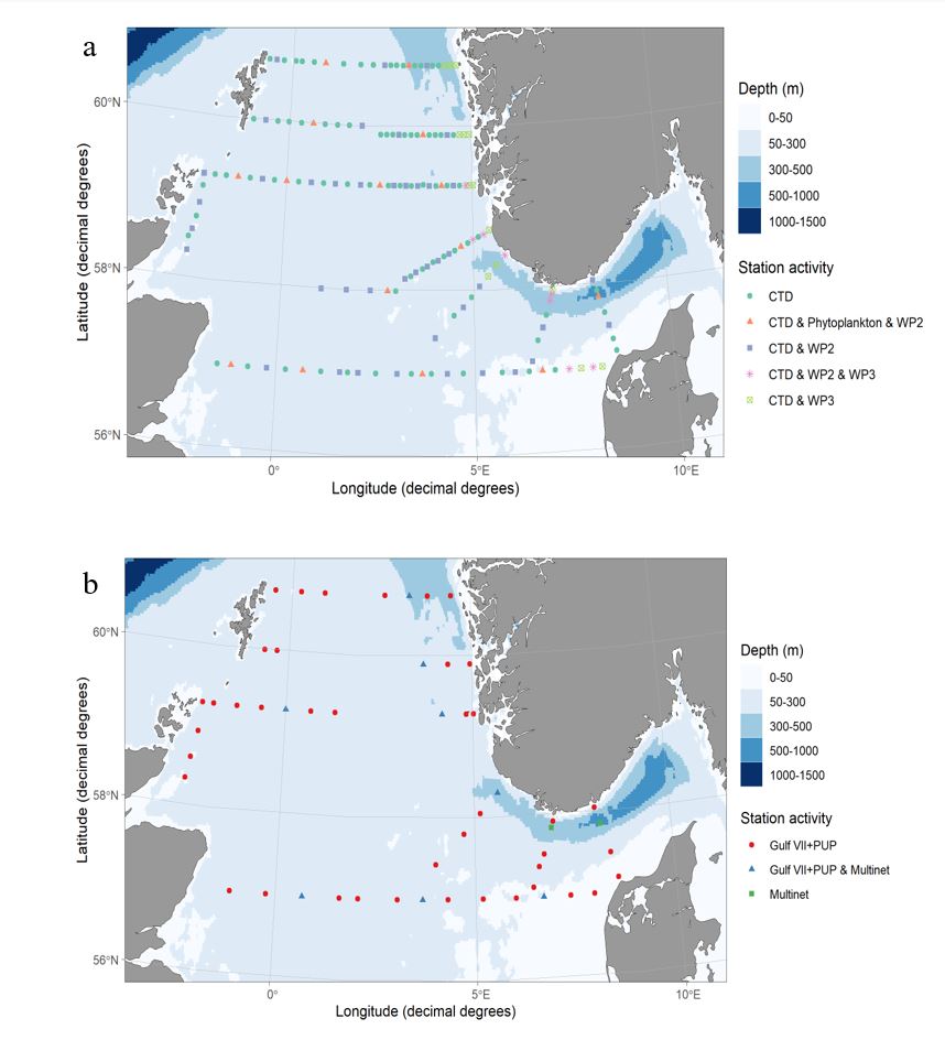
The cruise program was undertaken according to Table 3. Maps of the cruise activities and stations are presented in Figure 1a, b. Sampling was undertaken on a 24 hour basis.
Leg 1 (14 st April – 26 th April): The vessel left Bergen at 12:00 UTC on April 14 th 2022. At the beginning of the cruise before the start of the survey, we performed calibration for the flowmeters of both the GULF VII and the MultiNet Mammoth.
The survey started with the sampling of the Ferje-Shetland transect (60.45N 4.37E) at 20:00 of the 14.04.2022. The sampling continued with the Slotterøy mot W during which a front of bad weather was encountered forcing the crew to cancel 6 of the first 8 Gulf VII sampling. The survey continued with the sampling of the Utsira transect on the 17 th . High wind characterized also this transect forced the cancellation of two algae nets, one Multinet and 3 Gulf VII. Due to the time restrictions that the NSEC faced this year only half section of the Fair Isle-Pentland transect was surveyed. The cruise followed smoothly with the sampling of the Hanstholm-Aberdeen transect (57.00N, 8.11E-1.00W), Oksøy-Hanstholm, Egerøya mot SW, Lindesnes and Jærens rev SW + W .
Leg 2 (26 th April-12 th May) The second leg of the North Sea Ecosystem cruise 2022 was cancelled in order to share the vessel with the Tobis cruise which had no ship at disposal.
Despite the strong cut in the time provided to the North Sea Ecosystem Cruise, thanks to an efficient planning and the hard work of both the scientific and the crew personal, large area of the North Sea was cover by the survey. All the high priority transects were sampled avoiding an interruption in the long time series. However, the Skagerrak and the sea west of Denmark had to be taken out of the 2022 survey causing a gap in the monitoring series. The missing data affect not only the continuity of the monitoring of the North Sea but also other projects that count on samples collected during this cruise for their results. An examples are all the projects within the Coastal Program which use the coastal samples collected within the north sea transects.
A summary of the overall samples collected on the transects covered by the North Sea Ecosystem Cruise 2022 can be found in Table 6.
| Start | Stop | Activity | ||
|---|---|---|---|---|
| Date | Time | Date | Time UTC | |
| Leg 1 | ||||
| 14.04 |
12:00 |
Departure Bergen | ||
|
14.04 |
12:30 |
14.04 |
16:30 |
Calibration of Gulf and Multinett flow meters |
|
14.04 |
23:00 |
16.04 |
05:30 |
Transect “Feie – Shetland” |
|
16.04 |
12:00 |
17.04 |
20:00 |
Transect “Slotterøy mot W” |
|
18.04 |
00:00 |
19.04 |
18:30 |
Transect “Utsira-StartPoint” |
|
19.04 |
19:30 |
20.04 |
03:00 |
Transect ”Fair Isle-Pentland” |
|
20.04 |
12:20 |
22.04 |
11:00 |
Transect ”Hanstholmen-Aberdeen” |
|
22.04 |
12:00 |
22.04 |
17.30 |
Port Call Hanstholm |
|
22.04 |
18:30 |
23.04 |
04:30 |
Transect “Oksø-Hanstholmen” |
|
23.04 |
08:00 |
23.04 |
20:00 |
Transect “Lindsnes mot SSW” |
|
24.04 |
04:30 |
24.04 |
18:00 |
Transect “Egerøya Mot SW” |
|
24.04 |
20:30 |
25.04 |
22:00 |
Transect “Jærens rev SW + W” |
| 26.04 | 08:00 | Arrival in Stavanger | ||
Seawater temperature and salinity were measured at all stations with a SeaBird Electronics SBE911 CTD profiler fitted with a water bottle rosette.
Water samples for nutrient analysis (nitrate, nitrite, phosphate, silicate) were sampled from all CTD stations at all depths. From each depth 20 mL aliquots of sample water were collected in clean polyethylene bottles and added 0.2 mL chloroform, before storage at +4 ⁰C until further analysis at the Plankton Chemistry Laboratory at the Institute of Marine Research (IMR) in Bergen. Chlorophyll pigment samples (268 mL) were taken from eight depths between the surface and 100 m and collected on GF/F fiber glass filters. The filters were stored at -20 ⁰C to be analyzed for Chlorophyll-a and Phaeopigments (Chl-a, Phaeo) at the Plankton Chemistry Laboratory in Bergen.
Samples for phytoplankton community composition and abundance were collected from 21 preselected stations along the transects. Phytoplankton samples were collected using two methods, the Algae-net and CTD. Qualitative Algae-net samples were collected using a vertical net tow (10 μm mesh; 0.1 m 2 opening; 30-0 m), fixed with 2 ml 20% formalin and stored for future use. Samples for algal cell counts (100ml) were taken from 10 m CTD collected water and fixed in Neutral Lugol. Microscope counts were performed following the Utermöhl (1958) method on all CTD samples to quantify community composition and abundance at the Flødevigen Plankton Laboratory .
The majority of stations sampled for phytoplankton (20) were sampled during the NSEC and included paired CTD and Algae-net samples. One CTD sample was also collected during the Torungen-Hirtshals transect cruise (2022305).
Plankton samples for imaging analysis were collected at 38 selected stations along the standard North Sea transects. Samples were collected in parallel with phytoplankton and zooplankton microscopy samples to acquire a better understanding of whole North Sea plankton community structure. Water samples from plankton enumeration, identification and size structure analysis (1000-500 ml) were collected from the 10m CTD sampler bottle, fixed in 2% (fin. Conc.) acidic Lugol and stored in a dark refrigerated room (4⁰C). Post cruise analyses were performed at the Flødevigen Plankton Laboratory . Sampled were analyzed using a Flowcam VS-1 quipped with a 2x objective lens and a 800µm deep non-field-of-view flowcell (magnification = 20) , a flowcam 8400 laser equipped with a 10x objective lens and a 100µm deep field-of-view flowcell (magnification = 100). and a flowcam Macro with a 0.5x objective lens and a 5000µm deep field of view flowcell (magnification = 12).
Mesozooplankton were collected by vertical tows with WP-2 plankton nets (0.25 m2 opening; 180 μm mesh size) from the bottom to the surface, and from 200-0 m, bottom depth permitting. Additional stratified sampling of zooplankton was carried out by Multinet MAMMOTH (Hydrobios, 180µm, soft cod-ends). Oblique tows were made from 5 m above bottom while releasing nets at standard depths (Table 4)
| Depth strata | MultNet number |
|---|---|
| 0-bottom | 0 |
| bottom-400 | 1 |
| 400-300 | 2 |
| 300-200 | 3 |
| 200-150 | 4 |
| 150-100 | 5 |
| 100-50 | 6 |
| 50-25 | 7 |
| 25-0 | 8 |
Large medusae and ctenophores were removed from whole samples, and the displacement volume of each species was recorded. The remaining zooplankton sample was split in two parts by a Motoda plankton splitter: one part was fixed in 4% borax buffered formaldehyde for species identification and enumeration. The other half was used for estimation of biomass (dry weight): samples were fractionated into three fractions (180-1000µm, 1000-2000µm and >2000µm) and placed on pre-weighted aluminum trays, dried at 60°C for 24 hours and kept in a freezer until return to Bergen. From the >2000 μm size fraction euphausiids, shrimps, amphipods, fish and fish larvae were counted, and their lengths measured separately before drying. In addition, Chaetognaths, Pareuchaeta sp. and Calanus hyperboreus from the >2000 μm size fraction were counted and dried separately (but sizes not measured).
Samples were not split on the transect Hanstholm-Aberdeen, due to shallow depths and small sampling volumes. Instead, two WP2-tows were taken: 1/1 sample was fixed in 4% formaldehyde, and 1/1 sample was fractionated and dried for later biomass measurements. All dry weights were determined at the IMR plankton laboratory in Bergen after the cruise. Details on the sampling procedures are found in the IMR Plankton Manual (Hassel et al., 2019).
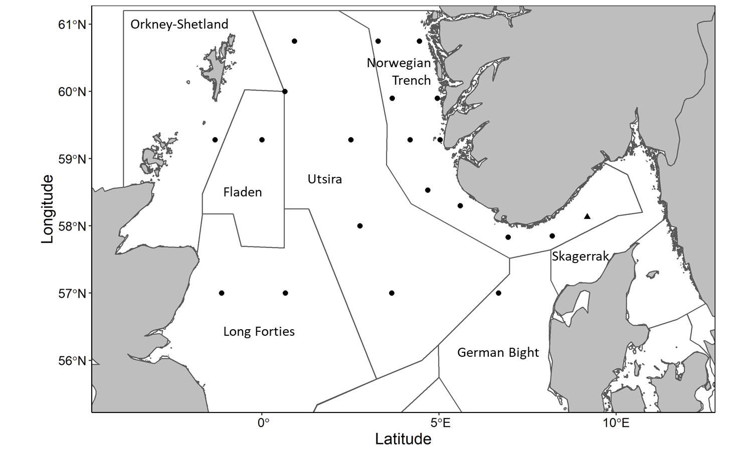
Sampling for fish eggs and larvae was undertaken at selected stations along each of the standard North Sea transects (Figure 1b) using a Gulf VII high-speed sampler (Nash et al. 1998) (76 cm frame). The sampler was fitted with a 40 cm diameter nose cone, a General Oceanics flow meter was fitted slightly off center in the nose cone (for quantities of water filtered) and a 280 µm mesh net. The sampler was towed at 5 knots in a double oblique haul to 100m depth or to within 10m of the bottom. All fish eggs and larvae were sorted from the samples at sea, sub-sampling being undertaken where necessary, and preserved in 4% seawater and Borax buffered formalin.
In addition, a PUP sampler (5 cm diameter nosecone with a General Oceanics flowmeter to determine the water volume sampled and a 80 µm mesh net) was fitted to the Gulf VII to provide samples of prey items for fish larvae. These samples were also preserved in 4% seawater and Borax buffered formalin.
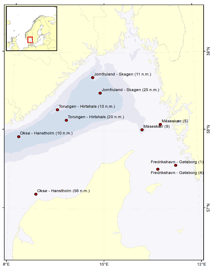
Water samples are collected yearly from 10 preselected stations in the Skagerrak (Table 5, Figure 2) for analyses of the radionuclide cesium-137 (Cs-137) (project number 15595). In 2022, the geographical coverage of the planned cruise was greatly reduced, and sample collection was reduced to the two stations at the Oksø-Hanstholm section (Table 5). Samples from the two stations at the Torungen-Hirtshals section were collected from “G. M. Dannevig” in June. At each station, 50 liters of seawater are collected from the ship’s seawater intake and filled directly into 25 L plastic cans. The samples are later analysed for Cs-137 at the Laboratory for inorganic chemistry at IMR, Bergen, according to the internal method “460 - Bestemmelse av Cs-137 i sjøvann” (MET.UORG.01-17). This is a modified version of the analytical procedure described by Roos et al. (1994).
Table 5. Station list. Samples collected April 2022 for monitoring of Cs-137 are indicated. Samples from the two stations at the Torungen-Hirtshals section were collected from “G. M. Dannevig” in June.
Monitoring of radioactive contamination in the Skagerrak is part of the national monitoring program Ra dioactivity in the M arine E nvironment (RAME), which is coordinated by the Norwegian Radiation and Nuclear Safety Authority (DSA) (e.g. Skjerdal et al., 2017; Skjerdal et al., 2020).
Monitoring of radioactive contamination in the Skagerrak is part of the national monitoring program Ra dioactivity in the M arine E nvironment (RAME), which is coordinated by the Norwegian Radiation and Nuclear Safety Authority (DSA) (e.g. Skjerdal et al., 2017; Skjerdal et al., 2020).
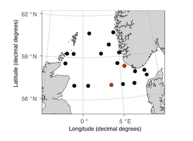
A small subsample (typically, 1/8 of the total sample) was obtained from the WPII nets at the (16 stations) or near-bottom MultiNet Mammoths (2 stations, Figure 3). The animals were immobilized using carbonated sea water then sorted under a stereomicroscope, and 200-400 animals were selected to create a “mock” sample. The sample was also supplemented with larger and/or rarer animals from the GULF net from the corresponding station. The body length of each animal was measured using the ZoopBiom digitizing system, and its biomass was estimated using a length-weight regression relationship published for the species (or a similar species). The samples were created to maximise diversity and varying contribution of various taxonomic groups in different samples. Two samples were created for each station: one was preserved in 100% Ethanol, and the other was rinsed in freshwater and placed on a pre-weighed aluminum tray, then dried at 65C for 24 hours. The two samples per station were designed to be very similar in quantity and composition, but not identical. In total, 33 samples were prepared from 18 stations (17 preserved via drying, and 16 in ethanol).
We used a 313-base pair fragment (“Leray” fragment) of the COI barcoding gene, which has been shown to be successful in recovering biodiversity at the species level in a wide range of marine invertebrates, including zooplankton (Wangensteen et al., 2018, Ershova et al., 2021).
| Transect | Station Number | Nutrients | Chlorophyl 1 | Phytopl. AbuC. | Phytopl. Net 30-0m | Flowcam Microplank | Flocam Mesoplank. | WPII Bottom-om | WPII 200-0m | WP III | Gulf VII | Multinet | Metabarcoding |
|---|---|---|---|---|---|---|---|---|---|---|---|---|---|
| Fedje-Shetland | 300-322 | 220 | 182 | 6 | 6 | 4 | 6 | 6 | 3 | 3 | 7 | 1 | 2 |
| Slotterøy mot W | 323-348 | 247 | 207 | 5 | 3 | 7 | 7 | 7 | 2 | 3 | 6 | 1 | 1 |
| Utsira mot W | 349-380 | 274 | 254 | 9 | 9 | 10 | 16 | 16 | 3 | 3 | 10 | 2 | 4 |
| Fair Isle - Pentland | 381-386 | 36 | 42 | 3 | 3 | 0 | 3 | 3 | 0 | 0 | 3 | 0 | 1 |
| Hanstolm-Aberdeen | 387-413 | 147 | 174 | 9 | 8 | 8 | 8 | 24 | 0 | 4 | 13 | 3 | 5 |
| oksø-Hanstholm | 414-420 | 54 | 46 | 3 | 2 | 5 | 3 | 3 | 1 | 0 | 3 | 1 | 2 |
| Lidesnes mot SSW | 421-427 | 65 | 54 | 1 | 1 | 1 | 4 | 4 | 2 | 3 | 4 | 1 | 1 |
| Egerøya mot SW | 428-435 | 65 | 60 | 1 | 1 | 1 | 5 | 5 | 1 | 3 | 5 | 1 | 1 |
| JærensRev | 436-456 | 181 | 161 | 6 | 6 | 3 | 10 | 10 | 0 | 3 | 0 | 0 | 1 |
| Sum | 1289 | 1180 | 43 | 39 | 39 | 62 | 78 | 12 | 22 | 51 | 10 | 18 |
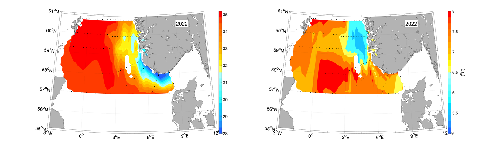
The hydrographic coverage of the survey area provides information on the main characteristics of the water masses in the northern North Sea and in the Skagerrak. The lowest surface salinities are typically found in the Skagerrak due to the Baltic outflow of low-saline waters through the Kattegat and the supplement of fresh water from local rivers along the Skagerrak coast. The resulting low-saline surface waters then follow the Norwegian coast westward out of the Skagerrak and northward along the coast, as the Norwegian Coastal Current (NCC). The shelf area in the northern North Sea is typically dominated by inflow of Atlantic water from the north (from the Tampen area) and from the west between the Orkneys and Shetland as the Fair Isle Current.
Based on the hydrographic measurements from the Ecosystem Cruise from the 14 th to 26 th of April 2022, the NCC can be identified in the resulting surface salinity map in the areas with the minimum values (Figure 4, left panel, blue and yellow colors). We also see relatively low temperatures varying between 5.5-6.5 o C in the NCC off the west coast of Norway, although the temperatures in the coastal areas off Rogaland and West of Agder is similar to what is observed in the northern and central North Sea (Figure 4, right panel). The northern North Sea is recognized as an area where relatively saline and warm water enters from both the north, from the Tampen area, and the west, as the Fair Isle Current.
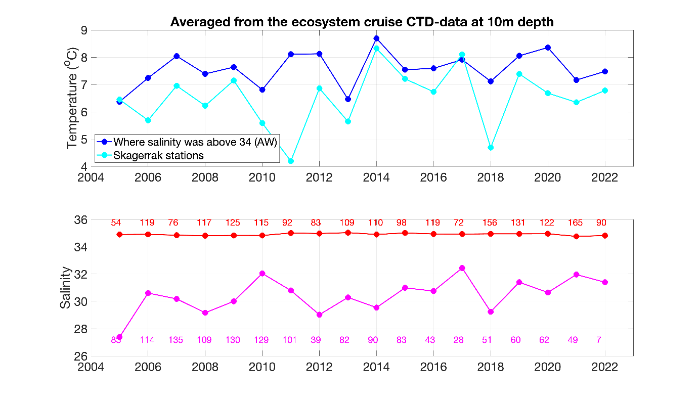
Compared to the long-term average based on all ecosystem cruises from 2005 until 2022, the Atlantic water temperatures in the northern North Sea in Spring 2022 were relatively (Figure 5). We cannot comment on the hydrographical situation in the Skagerrak since the transect between Oksøy/Norway and Hanstholm/Denmark was the only one included from that area due to the cut of the second leg of the ecosystem cruise.
Photosynthetic organisms in the ocean, such as phytoplankton, use sun light as their primary source of energy. Thus, they must live in the well-lit surface layer, the euphotic zone, in order to support the photosynthetic process. The light attenuation is an important parameter to determine the euphotic zone and can be influenced by the presence of both biotic and abiotic particles in the water. The depth of the 1% light irradiance gives an idea of the amount of particles in the water and the light available to phytoplankton. During the 2022 survey, the western and central part of the Utsira transect as well as the middle area of the Hanstholm-Aberdeen transect were characterized by the deepest 1% irradiance depth (Figure 6), suggesting a deeper mixed layer and low particles concentration. As matter of facts these areas correspond well with the lowest chlorophyll a concentration measured during our survey (Figure 8a).
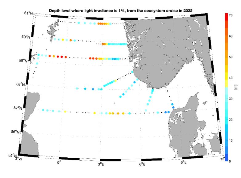
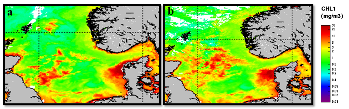
Figure 7 shows the evolution of Chlorophyll a concentration in the studied area during the period April 14 to April 26. The images are mean values over 8-day period. The satellites images show high accumulation of Chlorophyll a along all the coastal areas surrounding the North Sea. During the first 8 days of the survey plums of high chlorophyll concentration were observed in the western part of the North Sea (Figure 7a) while during the second half most of the Norths Sea Shelf area was characterized by high chlorophyll concentrations (Figure 7b). The most productive area during the all period surveyed was the western coast of Denmark which was sampled on the 22 of April by our crew.
During the 2022 North Sea ecosystem survey chlorophyll a concentration ranged between 0.07 and 6.42 µg/L with the highest concentrations recorded in the middle of the North Sea bank. Concentrations between 2 and 3 µg/L were also measured in the Northwest area and along the Danish west coast (Figure 8a). In general, high chlorophyll a concentrations were associated with low nutrient availability suggesting previous use by phytoplankton. More specifically, high total nitrate and phosphate were measured in the Northwest sector while along the Norwegian coast and west of Denmark dissolved inorganic nitrogen (DIN) and Phosphate were quite low (Figure 8b-c).
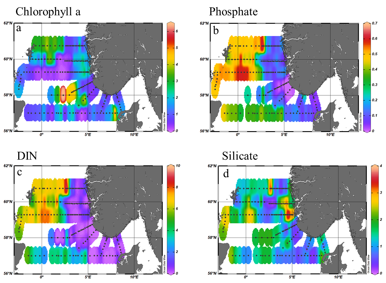
Silica on the other hand, presented higher concentrations on the west coast of Norway and east coast of Scotland and, along the Utsira transect while lower concentrations were measured along the southern Norwegian coast and in the northwest sector (Figure 8d). Surface s ilicate concentrations were <2μM at 40% of the stations visited. L ow silica concentrations were often associated with high abundance of d iatoms, the single user of silica, suggesting a depletion of silica had occurred to fuel diatoms growth.
Samples for phytoplankton community composition and abundance were collected from 21 preselected stations along the selected transects, covering multiple WGINOSE sub-regions (Figure 10).
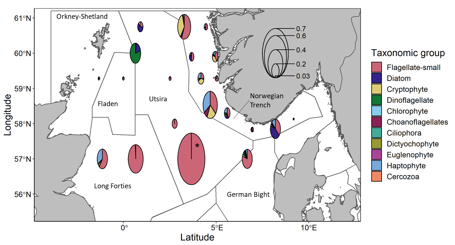
Based on microscopy counts, the North Sea microplankton community at an average station was numerically dominated by small flagellates (67%, 3.2×10 5 ± 6.2×10 5 cells ml -1 ) with smaller contributions from cryptophytes (9%, 4.2×10 4 ± 6.4×10 4 cells ml -1 ), diatoms (8%, 3.7×10 4 ± 6.5×10 4 cells ml -1 ) and haptophytes (8%, 4.0×10 4 ± 6.9×10 4 cells ml -1 ). The dominance of small cells is consistent with previous observations and may reflect an advantage in low nutrient environments. Spatial distribution within the North Sea showed that abundances were relatively low in the northwest stations (9.1×10 4 -5.7×10 5 cells ml -1 ), high in the south (2.7×10 5 -2.9×10 6 cells ml -1 ) and variable within the Norwegian trench (7.7×10 5 -6.1×10 4 cells ml -1 ) (Figure 11). Small flagellates comprised a large proportion of the communities at many stations, especially the high abundance southern stations along the Hanstholm-Aberdeen transect, accounting for 60-100% of the communities at those stations. Cryptophytes were abundant community members only within a subset of Norwegian trench stations. Dinoflagellates, which may include autotrophic, mixotrophic and heterotrophic species, comprised a large proportion of the community (79%) at only one station, located at the northwest edge of Utsira. Diatoms were numerically important community members at only a few stations without a single defined region. Variations in community composition have implications for food quality and can impact the flow of carbon to higher trophic levels.
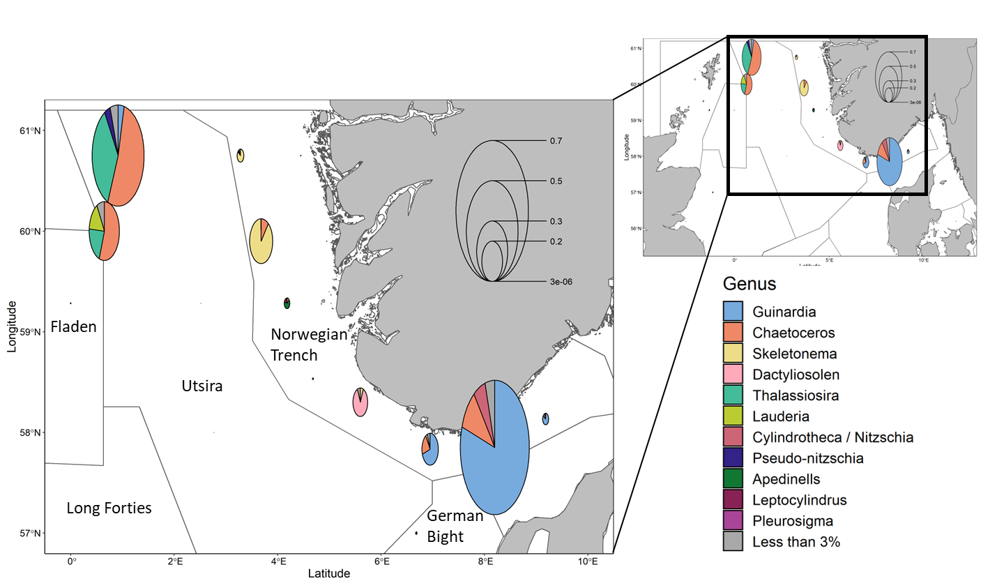
Diatoms are a major group within primary producers and can be used as indicators of environmental conditions. This group is thus examined at a high taxonomic level. Diatoms abundance was greatest in the northwest Utsira stations (1.1×10 5 -1.8×10 5 cells ml -1 ) and within a subset of the Norwegian Trench stations (7.2×10 3 -2.4×10 5 cells ml -1 ) (Figure 12). Community composition within the diatoms varied spatially. In the Norwegian Trench Guinardia spp dominated southern stations while Skeletonema spp was more important in the North. Utsira diatom communities differed from the trench and were comprised mainly of Chaetoceros spp. , Thalassiosira spp. and Lauderia spp .
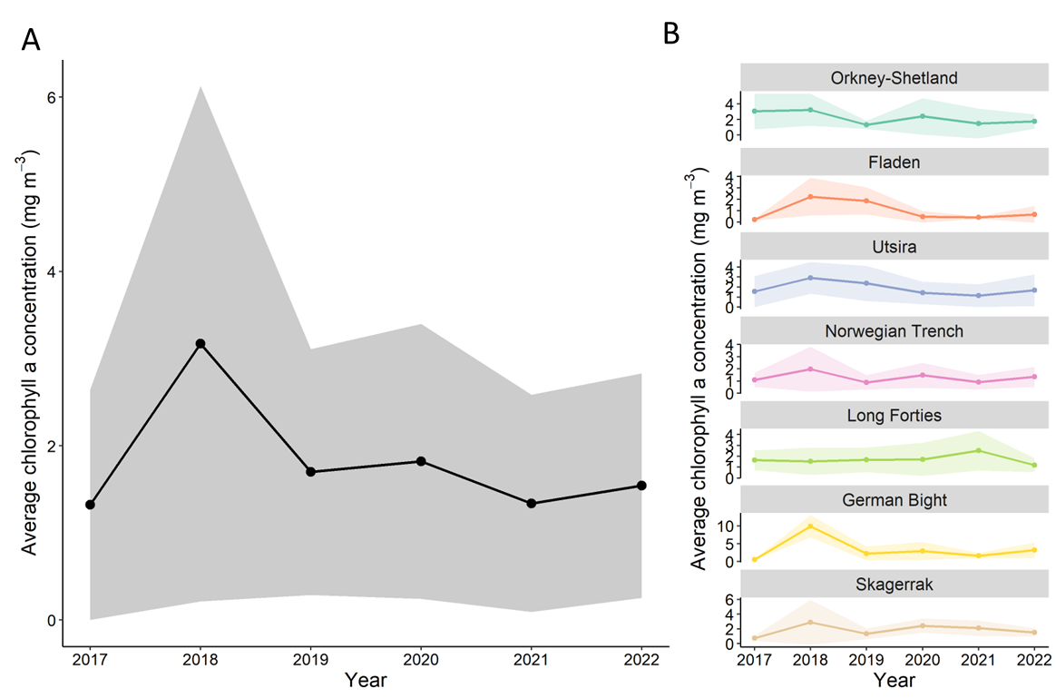
When compared to results from previous NESCs, the average concentration of microplankton was reduced in 2022 (Figure 13). Declines in average abundance were seen in small flagellates, diatoms, and cryptophytes which declined by 25%, 66% and 72% respectively relative to 2021.

In contrast, surface chlorophyll concentrations have remained relatively stable during the same period across the North Sea as well as within WIGNOSE sub-regions (Figure 14). Stable chlorophyll a values may be supported by photosynthetic groups not captured with these sampling methods such as single celled cyanobacteria or large, rare taxa. It is also possible that larger cells were relatively more important photosynthetic contributors in 2022, causing what may seem like a mismatch in the total chlorophyll and cell abundance.
Plankton samples from selected stations of fix transects have been analyzed though flow imaging systems (FlowCam). Taxonomic and functional determination were assigned though a machine learning approach. Using three different instruments we were able to analyze the plankton community structure in a size range from 5 till 2000µm.
With this analysis we have obtained a rapid assessment of the community structure and we were able to identify the main taxonomic groups: Flagellates, Diatoms, Heterotrophic/Mixotrophic protists, Calanoid copepods, Oithona sp., Nauplia and other copepods and other mesozooplankton.
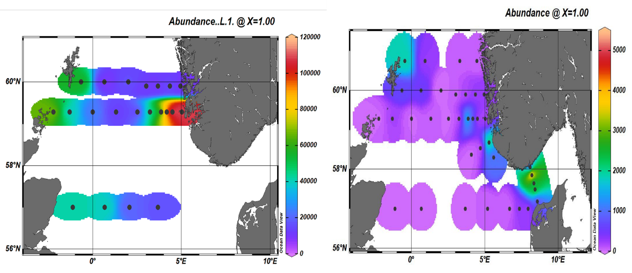
The smallest cells of the phytoplankton were detected with a FlowCam 8400 laser. Due to technical issues not all the samples were analyzed with this instrument however, despite the limited number of samples we detected higher concentrations of small flagellates at the coastal stations of the Utsira transect and along the Hanstholm-Aberdeen transect. Elevated concentrations were also registered at the northwest corner of the North Sea. Due to their larger size, diatoms can be detected with two instruments, the FlowCam 8400 and the VS-1. Data from the VS-1, show that diatoms were most abundant in the northwest sector of the North Sea and in the Norwegian trench. High concentrations were measured particularly along the Oxøy-Hanstholm transect (Figure 15b). These data correspond well with the microscopy analysis and show that, for a quicker not species-specific analysis this imaging-based technology can provide great information.
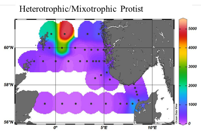
With this technology we were also able to obtain a better coverage of the North Sea for the zooplankton component. The smaller planktonic predators, the microzooplankton which are mostly heterotrophic and mixotrophic ciliates and dinoflagellates have not been consistently monitored till now. With the addition of the FlowCams to our instrumentation we were able to add this trophic level to our analysis and monitoring program. The highest abundances were measured again in the northwest sector in association with high phytoplankton counts (Figure 16).
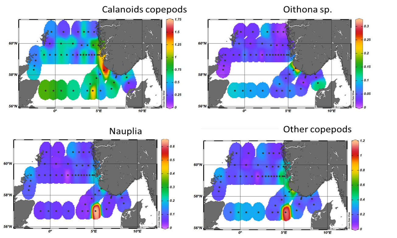
As for the mesozooplankton component (>180 µm) we were able to identify several groups: Calanoid copepods, Oithona sp., nauplia, other copepods and other mesozooplankton. The analysis shows that calanoids copepods were the most abundant group within mesozooplankton and that they were distributed in all the North Sea. However, the highest abundances were recorded in the Norwegian trench in association with deeper waters (Fig. 17a). The same coastal station on the Jærens Rev transect also registered the high numbers of Oithona sp. while nauplia, the larval stage of copepods, were quite abundant outside the west coast of Denmark.
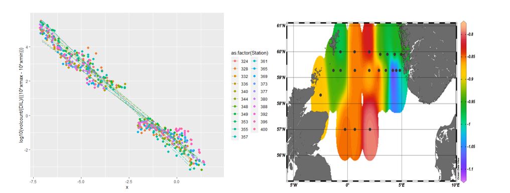
Combining the size data from the three FlowCams we are able to build plankton size structure analysis for the sampled stations. The steepness of the slope of the curves revels the higher or lower contribution of smaller cells to the plankton assemblage. Thus, the analysis reveals that the plankton community of the North Sea in spring 2022 was dominated by smaller plankton organisms at all stations (Figure 18, left panel). However, the slight differences in the slopes obtained for each station translate in different contribution of the different size classes to the plankton community. Thus, using the slope obtained for each station we can create maps that visually inform on the size class distribution in the North Sea: the warmer color represents less steep slopes and thus a higher contribution of larger organisms to the plankton community while warmer colors are associated with more steep slopes and thus smaller plankton (Figure 18, right panel).
Zooplankton biomass
Overall, the average zooplankton biomass for the whole survey area was 8.2 g m -2 which is above the long-term average of 5.5 g m -2 (2005-2021; Figure 19).
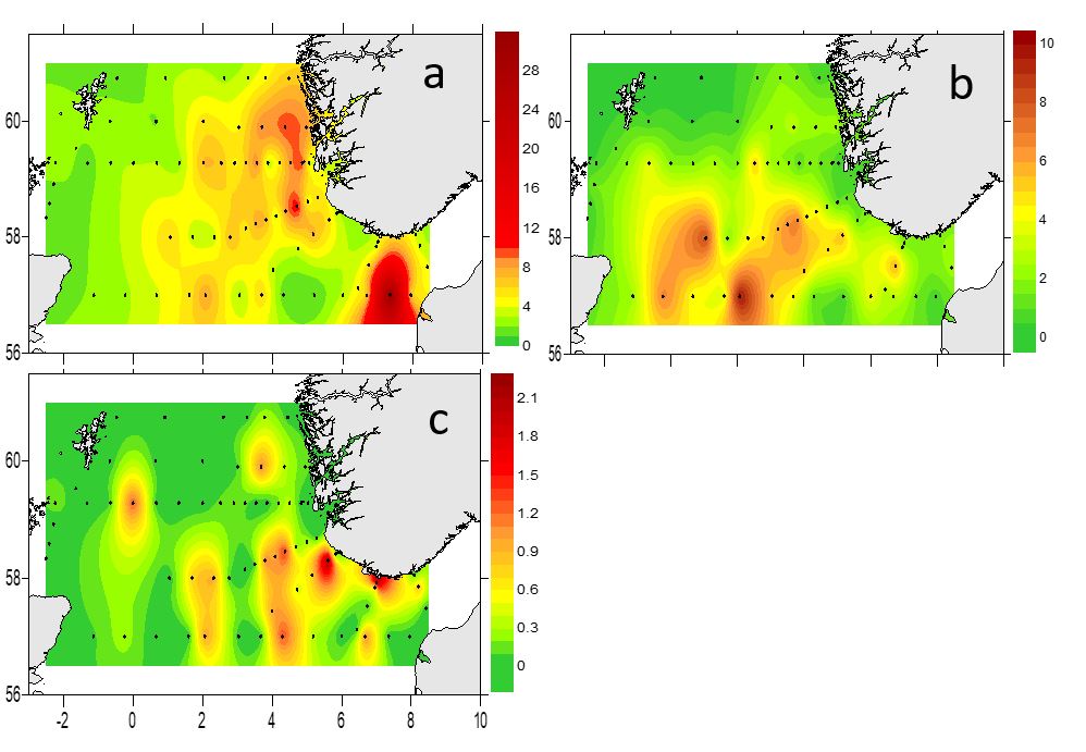
Depth integrated zooplankton biomass (g dry weight/m 2 ) in April 2022 is presented as total biomass (>180µm, Figure 20) and as three different size fractions (Figure 21a-c). The highest biomass values were registered in the central area, and on the Hanstholm-Aberdeen transect (maximum 34 g/m 2 , Fig 20). The 180-1000 µm size fraction (Figure 21a) contains small sized copepods ( Oithona sp, Pseudocalanus spp), juvenile stages of large copepods ( Calanus ) and benthic larvae. However, this fraction may also contain phytoplankton. The highest biomass values of this smallest fraction were observed on the Norwegian side and along the Hanstholm-Aberdeen transect. The 1000-2000 µm size fraction, which is dominated by Calanus spp., showed highest values in the central and southern part of the survey area (Figure 21b). The biomass of the size fraction >2000 µm was generally low, and with a patchy distribution (Figure 21c).
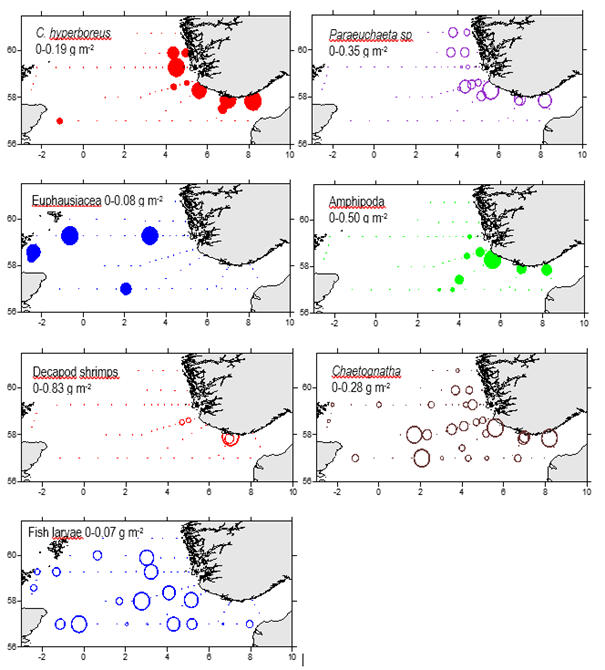
The biomass of single taxonomic groups, larger than 2000 µm are shown in Figure 22. The >2000µm size fraction contains a large variety of planktonic organisms from large sized copepods ( Calanus hyperboreus, Paraeuchaeta norvegica) to amphipods, decapod shrimps, and chaetognaths. Most of these groups were associated with the deeper waters in the Norwegian trench. Fish larvae and euphausiids however, had a wider distribution in the survey area.
Zooplankton taxonomic composition
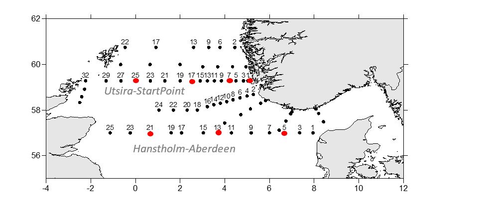
Species identifications and enumeration of zooplankton (WP2 tows) has been analyzed on selected stations along the two transects Utsira-StartPoint and Hanstholm-Aberdeen (Figure 23).
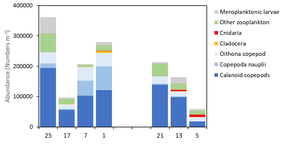
Copepods was the numerically dominant group of zooplankton across the transects Utsira-StartPoint and Hanstholm-Aberdeen (Figure 24). Higher densities of copepods were encountered on the western stations, numerically dominated by small copepods (Oithona and Pseudocalanus). Cnidarians ( Aglantha digitale and hydrozoa) were most numerous on the Danish side of the Hanstholm-Aberdeen transect. Other important groups were larvaceans (Appendicularia), pteropods ( Limacina retroversa ), euphausiids and meroplanktonic larvae. Crustacean larvae of several benthic decapod species (Brachyura, Anomura) were recorded in the samples but not identified to species level.
The contribution of different taxa to the copepod community is presented in figure 25. More in detail, Para/Pseudocalanus, Calanus spp and Oithona spp were the numerically dominating taxa. Temora longicornis was typically abundant in the near-shore stations towards Norway and Denmark (stations 1 and 5). Small numbers of the large species Paraeuchaeta norvegica, C. hyperboreus and Heterorhabdus norvegicus were found in the deeper waters of the Norwegian Trench (Utsira-StartPoint, station 7).
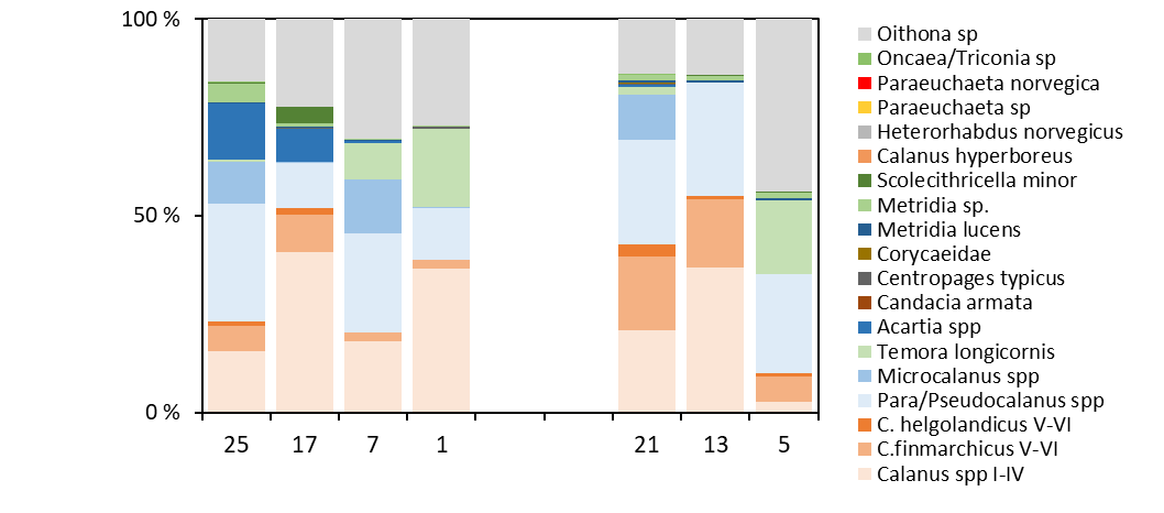
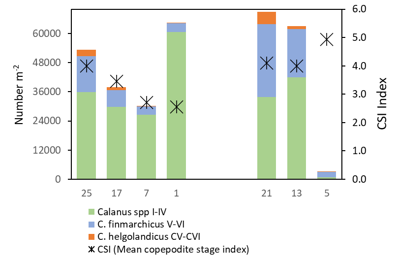
High abundances of Calanus spp were recorded on both transects, dominated by small copepodite stages (CI-CIV). Although C. finmarchicus and C. helgolandicus co-occurred across the survey area, C. finmarchicus was the numerically dominating species on all stations, comprising >80% of the Calanus spp CV-CVI (Figure 25). The highest proportion of C. helgolandicus were found on the easternrnmost station on the Hanstholm-Aberdeen transect (Stn 21).
To explore the stage composition of Calanus , the mean copepodite stage index (CSI) is presented in Figure 26 as an abundance-weighted mean stage (CSI=1 when all CI, and 6 when all adults). The CSI ratio varied between 2.5 and 4.9 which can be interpreted as variations in phenology in different parts of the surveyed area. CSI values less than 3 on the Utsira transects, suggests that Calanus was in an earlier phase of the seasonal reproduction in this area compared to stations further south on the Hanstholm-Aberdeen (CSI 4.1-4.9).
The Baltic Sea is the largest source of radioactive contamination to Norwegian waters today. The reason for this is that land areas around the Baltic Sea received significant amounts of fallout from the Chernobyl accident in 1986. Run-off from these contaminated land areas is transported with ocean currents from the Baltic Sea through the Kattegat to Norwegian waters. To monitor the supply of cesium-137 (Cs-137) to Norwegian waters, samples of seawater have been collected yearly since 2008 from the 10 stations shown in Figure 2. The coordinates for each station are listed in Table 5.
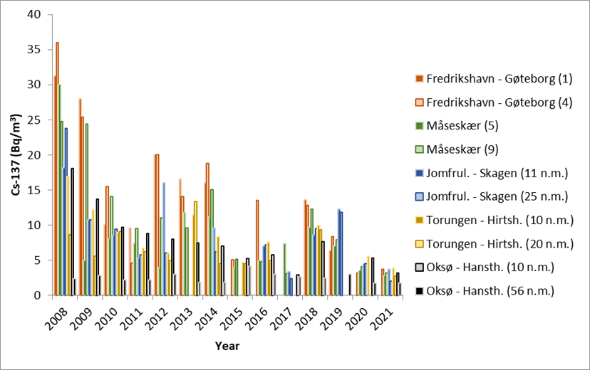
Results from 2008 to 2021 are shown in Figure 27. The samples collected in 2022 are not yet analysed. The highest activity concentrations of Cs-137 are, as expected, found at the Fredrikshavn–Gøteborg section, which is nearest the outlet of the Baltic Sea. The lowest activity concentrations are found at the Oksø-Hanstholm section. The activity concentrations of Cs-137 at Oksø-Hanstholm (56 n.m.) have been more or less constant in the period 2008-2021. This is as expected as seawater at this station has characteristics more like the North Sea. In 2021, the activity concentrations at all stations were below 5 Bq/m 3 for the first time since we started the monitoring in 2008.
Although there is a constant supply of Cs-137-contamination from land to the Baltic Sea, the data indicate a general decreasing time trend (Figure 27). This is mainly due to radioactive decay of Cs-137, which has a physical half-life of 30 years. Yearly variations in Cs-137 levels are due to variations in precipitation and run-off from land and oceanographic processes, among other things.
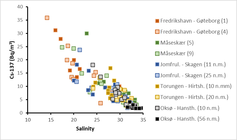
Figure 28 shows activity concentrations of Cs-137 (Bq/m 3 ) at each station plotted against salinity. There is a clear negative correlation between salinity and activity concentrations of Cs-137. The Baltic Sea has brackish water, and the salinity of its surface waters vary from 1–2 in the northernmost Bothnian Bay to around 20 in the Kattegat compared to 35 in the North Sea. Thus, low salinity implies larger degree of “Baltic Sea characteristics”. Higher salinity implies larger degree of “North Sea characteristics”. This generally agrees with our Cs-137-results.
Sequencing of mock samples revealed no differences in recovered DNA concentration, sequencing depth or species counts between ethanol and dry samples (Figure 29). This suggests that samples dried at 65 degrees C can be just as good as preserving DNA as ethanol preservation. However, certain caveats need to be noted before this result is extrapolated onto the dry weight samples typically taken on IMR cruises. First, the quantities of preserved material in this study were much smaller than is in a typical dry weight sample taken for biomass, which ensured quick and even drying. Second, the samples were removed promptly after 24 hours, while the biomass samples are typically left in the oven until the end of the cruise or until the oven fills up. Finally, these “mock” samples were not subjected to a second heating cycle to remove any residual moisture, as is done post-cruise prior to weighing.
The visual identification yielded a total of 59 unique holoplanktonic and 16 meroplanktonic species/taxa across all samples. Metabarcoding identified 76 holoplanktonic and 107 meroplanktonic species/taxa, which included all but 3 of the species identified visually (two appendicularians and one monstrilloid copepod), as well as numerous additional species of hard-to-identify crustaceans, hydrozoan jellyfish and larvae of benthic animals. For example, the group Pseudo/Paracalanus spp. consisted of 5 different species found in varying proportions at different stations, of which Paracalanus parvus was the numerically dominant one.
On a sample-to-sample basis, typically 90-95% of registered species/taxa were recovered via metabarcoding, with the number of “false negatives” (species not detected via metabarcoding) never exceeding 2-4 species. However, the percentage of “false positives” (species that were identified via metabarcoding but were not detected visually) was also quite high, on some stations making up 40-50% of the total species. When the detection threshold was dropped to 0.01% of total sequences, the percentage of false positives was reduced to less than 10% across all stations, but the percentage of false negatives rose, as some of the “real” species began to fall under that threshold. As metabarcoding is an extremely powerful tool and given enough sequencing depth can detect trace amounts of DNA (including residual fragments of organisms or stomach contents of other species), this result highlights the need to be mindful of the detection threshold when obtaining biodiversity estimates via metabarcoding, both in terms of false positives and false negatives.
When examining the sequencing data quantitatively, strong correlations were observed between biomass and sequence counts for most taxa. However, for many species and taxa, the ratio between the number of sequence reads and biomass was significantly different from 1, meaning that they were consistently either over- or under-represented in the sequencing data relative to their biomass contribution to the sample. The slopes of the regression lines were then used to introduce linear conversion factors to bring the relationship closer to 1:1. These linear conversion factors were applied across the entire dataset (Figure 30). Our data confirms that m etabarcoding data can be used in a quantitative way as a proxy for biomass, and applying species- or taxa-specific conversion factors can maximize comparability between these two measures. These relative values can then be converted to absolute biomass estimates by multiplying the % of the sequence reads by the total biomass of the sample.
The sampling of North Sea during the ecosystem cruise 2022 was strongly reduced due to the need to accommodate a Tobis survey. Despite the reduced time available the hard work of crew and scientific personal repaid with samples collected from all the highest priority transect plus additional transects, covering large sectors of the northern part of the North Sea.
The collaboration between the two IMR projects, Monitoring of climate and plankton in the North Sea Skagerrak (IMR 14920) and Early life history dynamics of North Sea Fishes (IMR 14917) provide a comprehensive overview of the distribution of phytoplankton, microzooplankton, zooplankton and fish species in the Northern North Sea and Skagerrak. Combining data on composition, distribution, abundance and carbon budget of phytoplankton, microzooplankton and zooplankton with species composition and distribution of fish eggs and larvae provide essential and unique information on the prey field and the bottom up drivers that affect survival and good development of the early life history stages (eggs and larvae) of a wide range of commercially valuable and non-commercial species. Using these data in a modelling effort will improve our predictive power and management effort.
We greatly appreciate and thank the masters and crew onboard RV Johan Hjort for outstanding collaboration and practical assistance at the North Sea Ecosystem cruise 2022. We are indebted to all the participants of the North Sea Ecosystem Cruise 2022 for their valuable work during collection and processing of samples and to all the technicians who help with the postprocessing of the samples in the Labs.
Ershova E.A., Wangensteen O.S., Descoteaux R., Barth-Jensen C., Præbel K. (2021) Metabarcoding as a quantitative tool for estimating biodiversity and relative biomass of marine zooplankton. ICE S Journal of Marine Science https://doi.org/10.1093/icesjms/fsab171
Roos P., 1994. Comparison of AMP precipitate method and impregnated Cu 2 [Fe(CN) 6 ] filters for the determination of radiocesium concentrations in natural water. Nuclear Instruments and Methods in Physics Research Section A: Accelerators, Spectrometers, Detectors and Associated Equipment. Volume 339, Issues 1–2, 22 January 1994, Pages 282-286
Skjerdal, H., Heldal, H.E., Gwynn, J., Strålberg, E., Møller, B., Liebig, P.L., Sværen, I., Rand, A., Gäfvert, T., Haanes, H. (2017). Radioactivity in the Marine Environment 2012, 2013 and 2014. Results from the Norwegian National Monitoring Programme (RAME). StrålevernRapport 2017:13. Østerås: Norwegian Radiation Protection Authority.
Skjerdal, H., Heldal, H.E., Rand, A., Gwynn, J., Jensen, L.K., Volynkin, A., Haanes, H., Møller, B., Liebig, P.L., Gäfvert, T. (2020). Radioactivity in the Marine Environment 2015, 2016 and 2017. Results from the Norwegian Marine Monitoring Programme (RAME). DSA Report 2020:04. Østerås: Norwegian Radiation and Nuclear Safety Authority.
Utermöhl, H. 1958. Zur Ver vollkommung der quantitativen phytoplankton-methodik. Mitteilung Internationale Vereinigung Fuer Theoretische unde Amgewandte Limnologie 9: 39.
Wangensteen O.S., Palacín C., Guardiola M., Turon X ( 2018 ) DNA metabarcoding of littoral hard-bottom communities: high diversity and database gaps revealed by two molecular markers . PeerJ 6 : e4705 https://doi.org/10.7717/peerj.4705