Rapporten dokumentere eit arbeidsmøte I COGMAR og CRIMAC prosjekta om automatisk målklassifisering av akustiske data. Føremålet med arbeidsgruppa var todelt. I den første bolken gav partnarane ei oversikt over kva dei held på med innan fagfeltet. Først gav vi ei oversikt over bruk av maskinlæring på automatisk målklassifisering av akustikkdata. Maskinlæringsmetodar, og spesielt djuplæring, er i bruk på mange tilsvarande felt, i tillegg til identifisering av mål frå fiskeriakustikk. Den andre føremålet var å gje deltakarar med maskinlæringsbakgrunn ei innføring i fiskeriakustikk og diskutera korleis vi kan etablera data standardar for å kunne effektivt samarbeida. Dette inkluderer datastandardarar, standard prosesseringssteg og algoritmar for effektiv tilgang til data for maskinlæring Resultatet frå diskusjonane vart delt med arbeidet i ICES mot ein data standard innan fiskeriakustikkmiljøet.
Fiskeriakustikk og akustisk målklassifisering
— Rapport frå COGMAR/CRIMAC arbeidsmøte om maskinlæring og fiskeriakustikk
Rapportserie:
Rapport fra havforskningen 2021-25
ISSN: 1893-4536
Publisert: 15.06.2021
Prosjektnr: COGMAR, CRIMAC
Forskningsgruppe(r):
Demersal fish
,
Pelagic fish
,
Acoustics and Observation Methodologies
Program:
Marine Processes and Human Impact
Approved by:
Research Director(s):
Geir Huse
Program leader(s):
Frode Vikebø
English summary
Sammendrag
This report documents a workshop organised by the COGMAR and CRIMAC projects. The objective of the workshop was twofold. The first objective was to give an overview of ongoing work using machine learning for Acoustic Target Classification (ATC). Machine learning methods, and in particular deep learning models, are currently being used across a range of different fields, including ATC. The objective was to give an overview of the status of the work. The second objective was to familiarise participants with machine learning background to fisheries acoustics and to discuss a way forward towards a standard framework for sharing data and code. This includes data standards, standard processing steps and algorithms for efficient access to data for machine learning frameworks. The results from the discussion contributes to the process in ICES for developing a community standard for fisheries acoustics data.
1 - Workshop format
The workshop was organized in two steps, were the first part was a mini conference on the use of machine learning methods on fisheries acoustics methods from the partners in the COGMAR and CRIMAC projects. The second part was a hands-on training session/hackaton on understanding, reading, and processing acoustic raw data.
The mini conference was a series of presentations of the approaches the different partners and institutions have used on fisheries acoustics data. The talks ranged from the recent advancement on using machine learning (ML) methods to the need for a framework for cooperation, data and algorithm sharing. The latter is linked to the ongoing efforts in ICES to develop a standard for acoustic data, and efficient connection to deep learning frameworks like Keras, Tensorflow and Pytorch, among others. The mini conference was held online November 1st, 2020.
The hackaton was organized December 7th- 11th 2020. The hackaton was a combination of small meetings, working in groups and training sessions on various aspects of reading, understanding and processing acoustic raw data.
2 - The mini conference
The mini conference was a series of presentations of the approaches the different partners and institutions have used on fisheries acoustics data. The talks ranged from the recent advancement on using ML methods to the need for a framework for cooperation, data and algorithm sharing. The latter is linked to the ongoing efforts in ICES to develop a standard for acoustic data, and efficient connection to deep learning frameworks like Keras, Tensorflow and pytorch, among others.
2.1 - LSSS and initial krill school detection by deep learning
Inge Eliassen and Junyong You gave a presentation of the Large Scale Survey System (LSSS) and presented initial work on using deep learning methods on krill school detections. They used screen shot images from LSSS as input to a U-net algorithm and Mask-RCNN and were experimenting with a RetinaNet architecture ( Figure 1 ).
2.2 - Supervised learning and adding additional information to the classifier
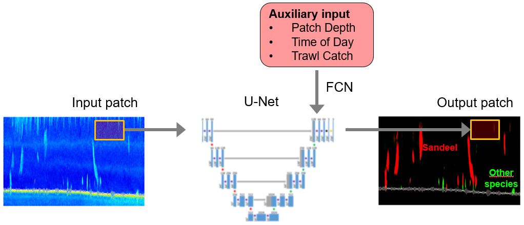
Olav Brautaset presented the work on using the U-net algorithm on the sand eel data (Brautaset et al. , 2020). The continuation of this work includes addressing variations in ping rate, falsely detected high energy pixels, and how to include auxiliary information to the network ( Figure 2 ). All these approaches show an improved performance of the network.
2.3 - Semi-supervised deep learning approach using self-supervision
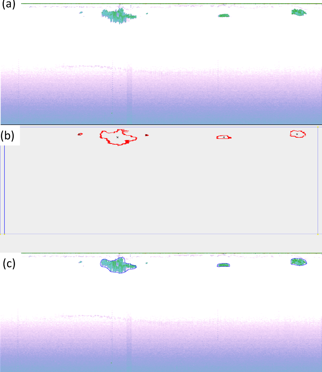
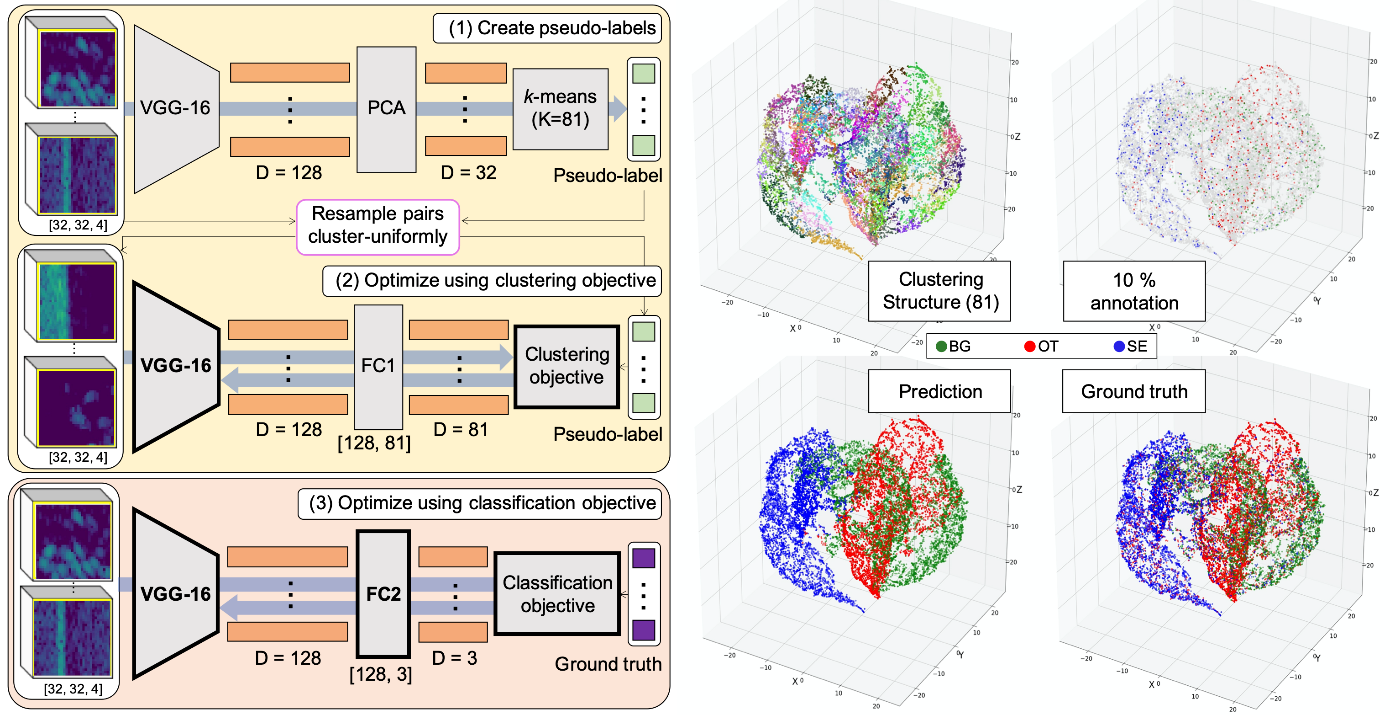
Changkyu Choi presented a semi supervised approach for classifying the sand eel data. He showed that a similar performance could be attained with only a subset of the labels. The idea is that all the data is used to learn a unsupervised representation for the data, and the labels are then combined in subsequent steps ( Figure 3 ).
2.4 - Unsupervised deep learning
Håkon Osland is working on unsupervised methods to cluster acoustic data into different classes. this approach is valuable for learning the structure and representation of large amounts of data. He has been experimenting with generative adversarial networks for establishing a lower dimensional representation of the data.
2.5 - Clustering drop sonde data
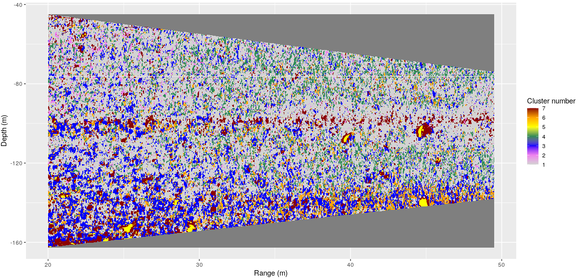
Tom Van Engeland is working on fine detail data from a drop sonde system. He is working on clustering techniques to establish different acoustic classes from the data ( Figure 4 ), and he is interested in whether the diversity of these classes can be used to address biodiversity in the area.
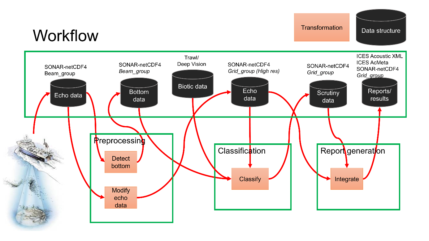
2.6 - IMR estimation workflow
Sindre Vatnehol and Ibrahim Umar presented the IMR data processing pipeline for fisheries advice. They emphasized the need to independent quality metrics on several levels, both on assessment results, survey indices, as well as finer scaled metrics. These metrics can be used for testing the sensitivity to different algorithms and parameters on and are useful for evaluating the different approaches in practice. They also emphasized the need for a data standard for the classification mask and the pre-processed data.
2.7 - Kongsberg processing pipeline
Arne Johan Hestnes presented the survey system that Kongsberg have been developing on top of their Kognifai platforms. We intent to use this platform for testing different classification algorithms. The platform supports docker images, and we intend to use that for testing and deploying different processing algorithms.
2.8 - General discussion
The work so far has been focused on traditional multiple frequency approaches using historical data. How to transfer this to broad banded data is an important step in the way forward, and the next steps will be to transfer that knowledge to cases where we start exploring the broad band spectrums.
The work so far has focused mostly on the Sand Eel survey since that have been made available for the participants, but it is important to move ahead with other surveys to ensure that we develop methods that are robust and scalable. The sand eel survey is also different to several other surveys in the sense that every school is manually labelled, whereas it is more common to allocate backscatter over a distance in other surveys. It is important that we include these other surveys to ensure that we develop methods that are general enough to tackle a broad range of problems.
The work presented have mainly focused on pixel based or patch-based predictions. This is the common approach for image analysis, but for acoustic trawl surveys, the backscatter itself is the key parameter. This means that low backscatter values are less important to get right than high backscatter regions. Weighing high intensity background images, like presented by Olav Brautaset, is an important step to reduce the overall error.
Different diagnostic tools need to be developed. These tools range from directly evaluating pixel wise annotations to the test set, via integrated backscatter over a distance, e.g. a transect, evaluating the performance metrics on the overall survey, and to effects on the assessment model results. These approaches can be used both for training, validation and testing. The latter is more relevant for testing since it requires larger computing resources. Sindre Vatnehol presented a few alternatives on how to move this forward, including different metrics to evaluate the consistency of a survey series.
The uncertainty in the acoustic target classification is not commonly included in survey estimates, but this constitutes an important source of uncertainty in the global estimate. The sensitivity to different classifications practices or algorithms can be analyzed and we can analyze the error propagation based on these uncertainties. This will be an important input to the survey estimation step, and the following assessment models.
2.9 - Discussion on collaboration and data standards
To make data available for the consortia and to ensure efficient collaborations across partners, the first step is to refine standards for exchanging data and algorithms between different computing modules. To steer the efforts, the existing pipeline will be used as a prototype. This pipeline consists of the manual classification from LSSS ( Figure 1 ), the preprocessing and classification pipeline developed by IMR and NR (Brautaset et al. , 2020), the IMR data processing pipeline, and the Kongsberg processing and scheduling platform.
The data standard should contribute to the efforts of the ICES working group on Fisheries Acoustics, Science and Technology (WGFAST) in developing a common data convention1, and details on how to contribute can be found there.
As a part of the ICES convention, a convention for interpretation masks is required. This information should contain the manual annotations and should cover content similar to the LSSS work files and the Echoview EV files. Code to read the LSSS work files exist2. A review of different data models has been performed3, and a test implementation exist4. There is also code that run the predictions from the U-net algorithm, write the test version of the masks, and wrap it up in a docker image5. We need to test this and see if it is sufficient for our purposes. The goal is that everyone that creates models for acoustic target classification should write this format to allow for testing the predictions through the Kongsberg system and in the IMR processing pipeline.
The interpretation mask is used in combination with (preprocessed) raw data to generate the integrated backscatter. These data have an established data standard that we need to adhere to. Both Echoview and LSSS supports this standard, and it is the input to the IMR processing pipeline. We have code that can read the proposed interpretation mask convention and post it to LSSS, and then use the LSSS infrastructure to generate the output. The process is rather slow when applied to a full survey, and alternatives are to write the work files or to generate a standalone light weight integrator.
Python is one of the most commonly used programming languages within machine learning, and shared data access code base for accessing acoustic data and annotations are needed. The python libraries accessing the data formats should be cloud friendly, and the internal representation in python should be able to efficiently use common machine learning frameworks, like Keras, TensorFlow and PyTorch. Two python-based packages that can read acoustic raw data are available. Pyecholab6 has support for low level reading of acoustic data, and echopype7 that supports net cdf exports and zarr data files, that are a cloud friendly format. There is also a possibility to write python-based API’s on top of the LSSS pre-processing code.
For implementation in Kongsberg and IMR’s data processing pipeline, it is recommended to set up docker images for the different models and adhering to the input and output data models. A first version of a docker image for the preprocessor and the U-net classifier have been developed8 That way, we can deploy the different models at a range of different platforms, both in the cloud and on platforms that are collecting data.
3 - The hackaton
3.1 - Objectives
To follow up on the recommendations from the one-day workshop, we set up a hackaton with the following objectives:
Objective 1: Learn how to read (and understand) acoustic data from single beam echosounders
The COGMAR and CRIMAC teams consists of people with skills across a wide range of fields, including fisheries acoustics, machine learning, statistics, etc, and the first objective was to get people familiar with the field of fisheries acoustics and to get hands on experience in reading and processing data. We use python as the language since most ML frameworks have good API’s in python.
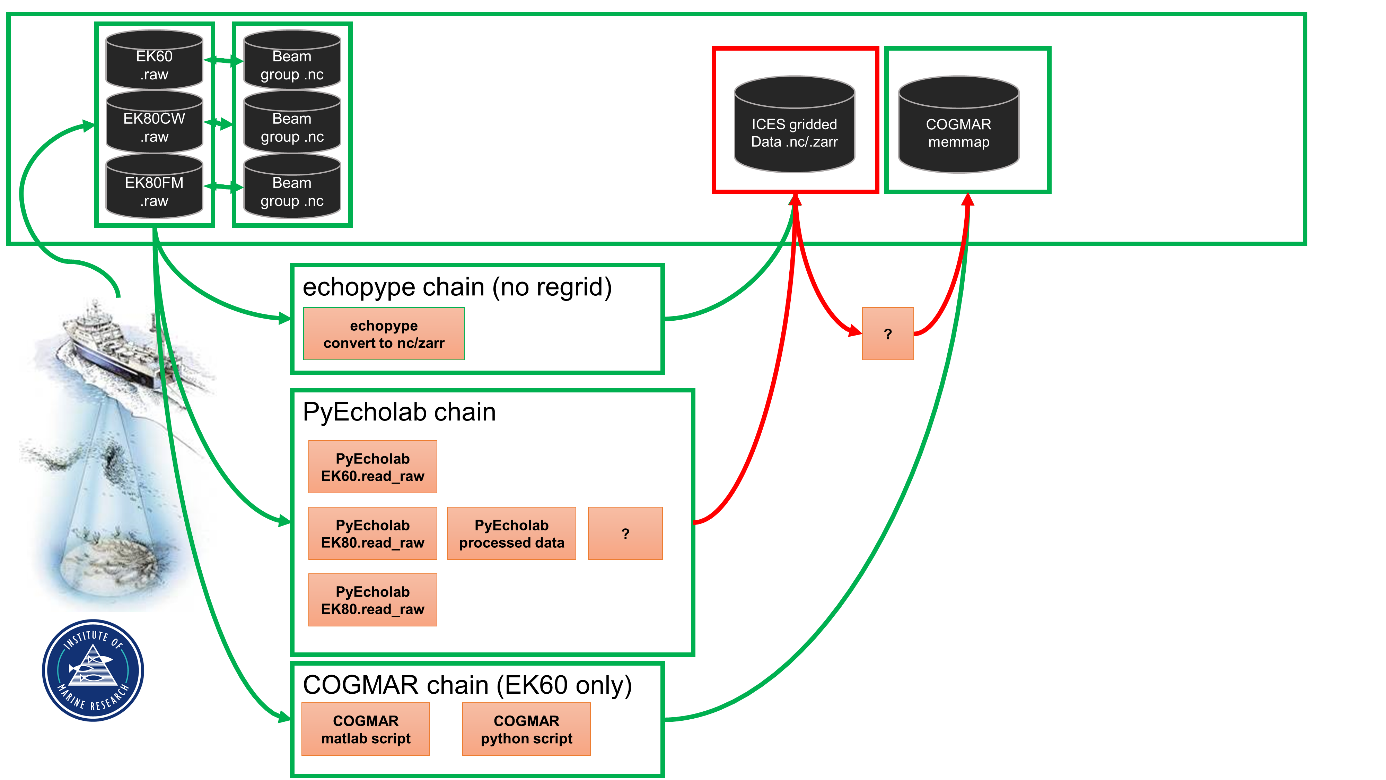
Objective 2. Code a pipeline from .raw to a gridded format
The first step in a processing pipeline ( Figure 5 ) is to read the data and cast it into a format that can be read by modern machine learning libraries. An important part of this process is to provide input to the standardization process in ICES. The objective was to discuss how to best prepare the data for the ML framework. These objectives do not cover the full pipeline, and that will be the topic for future workshops.
3.2 - Questions that you have had on acoustic data from echosounders, but never dared to ask
One of the main objectives was to bring participants with backgrounds in computer science up to speed on fisheries acoustics. To address this objective, we asked the participants after the symposium to list things that they did not understand or that were unclear. The following is a summary of answers to frequently asked questions that arose in this process.
3.2.1 - What is in the raw data?
The raw data from the split beam multi-frequency echo sounders (EK60) provide sampled backscattered energy together with athwartship (sideways) and alongship angles for each time step (ping). The angles are calculated by the phase difference between quadrants on the transducer face. The sampling rate and maximum range may vary between individual transducers, and may change between pings, and ping rate may vary over a survey transect. Data from individual pings may be missing due to intermittent system failures. As a result, the raw data will in general not fit directly to a time-range array. There are different ways of reading these data into python (Figure 6).
The EK80 split beam broadband echosounder has a continuous wave (CW, similar to EK60 but with higher sample rates) and a frequency modulated (FM) mode. The raw data from the EK80 in FM mode provides four channels of complex numbers, where each channel is from one quadrant of the transducer. The complex number denotes samples and the phase of the signal for each quadrant. In CW mode, these data can be processed to obtain data that correspond to the EK60 format, i.e. sv by range and angles from the phase differences between the channels. Note that the sample frequency is higher than for the EK60, but the data is still limited by the pulse length and remains similar. In FM mode, a chirp pulse is transmitted. This is a tone that change in frequency by time, and different sweeps can be configured. This also provides raw backscatter in four channels, but these data can be passed on to FFT algorithms to resolve the frequency domain. The data can be converted to a time-range-frequency grid per frequency channel after using the FFT.
The .raw files used by both EK60 and EK80 contains sequences of objects, referred to as ‘datagrams’. Each datagram starts with a length in bytes, the type (four ASCII letters, the last a digit signifying version), timestamp (two integers, alternatively, one long integer), the contents, and finally the length again as a sanity check. An EK60 file starts with a CON0 configuration datagram, followed by RAW0 datagrams each containing signal from one ping and one transducer/frequency. EK80 uses XML for configuration, and has an assorted number of new types (e.g. separate MRU datatype for heave/pitch/roll).
3.3 - Reading EK80
3.3.1 - Comparing EK80 readers between ESP3, pyecholab and LSSS
We tested different readers to see if there are differences in the initial data processing. An initial test showed some discrepancies ( Figure 7 ).
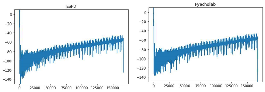
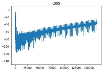
The subgroup kicked off by installing and getting familiar with the pyEcholab package and LSSS. There were differences between the packages, and it seems like ESP3 and pyEcholab interpret the data incorrectly, and likely contain (some of) the same processing errors.
The background material for looking into this is the documentation of the EK80 interface9.
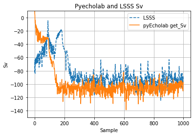
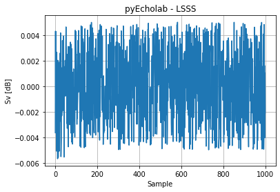
An EK80 file with data collected in broadband mode (38, 70, 120, 200 kHz) and narrowband (18, 333 kHz) was selected as a demo data set for testing. This file was collected with GO Sars during the first CRIMAC cruise. The file was selected as it’s reasonably small and collected using the latest version of the EK80 software (Nov 2020). Ping number 15 was selected for initial comparison of Sv from LSSS and pyEcholab. The first 1000 samples show some discrepancies between LSSS and pyEcholab ( Figure 8 ).
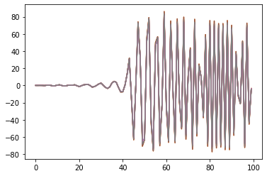
The complex values from the EK80 files were read per sector by LSSS and pyEcholab, allowing for a step by step process to identify discrepancies. The Raw complex values ( Figure 9 ), as read by pyecholab corresponds to LSSS and seems ok. A systematic comparison of the LSSS implementation and the pyEcholab code (EK80.py) was then performed, and in the following analysis three discrepancies were found in calculations of pulse compressed Sv compared to Simrads description on how to calculate pulse compressed Sv:
-
pyEcholab uses gain at the nominal frequency. This should be at the centre frequency.
-
pyEcholab uses psi at the nominal frequency. This should be at the centre frequency.
-
\tau_eff uses the signal, and not the autocorrelated signal.
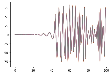
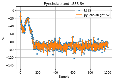
By applying these three changes to the pyEcholab code base, the results from LSSS and pyecholab are similar ( Figure 10 ). The modification was implemented in an “ad hoc” manner for the Hackaton, and needs a proper implementation, reading the relevant values from the raw file. The most recent update of the pyEcholab package have adopted these changes.
In addition there are two differences between LSSS and pyEcholab, which are not errors but more conventions to be agreed upon:
-
Should negative range values be plotted? LSSS keeps all data while pyEcholab only keeps positive values
-
pyEcholab : range=max(1,range), LSSS: range=max(sampleDistance, range)
3.4 - A ML friendly convention for echosounder data
Multifrequency echosounder data are stored in arrays per frequency, but machine learning libraries typically work on tensors. There has been an effort within ICES to move forward with a standardized format, and this part of the workshop reviewed the proposed standard for raw and processed echsounder data and provided input to the ICES process.
3.4.1 - The COGMAR “Echogram” class
The COGMAR project used the Sand eel survey as a test case and developed a ML friendly proprietary data format for the raw files and the label files from LSSS. Each pair of .raw and associated label is in this context called an “echogram”. This is a working processing pipeline and serve as a starting point for the discussion. The intention is to adapt this pipeline to the new format. The converted data from each raw file (echogram) are stored in separate directories ( Table 1 ).
The echogram class regrid the data into a tensor based on the grid for the 38kHz channel. Although the different frequencies are stored as separate files, they are aligned in ping and time.
| File name | File type | Data structure | Data type | Description | |
| Acoustic data | data_for_freq_18 | .dat | array(y, x) | float | Echogram data interpolated onto a (range, time) grid, common for all frequencies. Not heave corrected. Stored as numpy.memmap. |
| data_for_freq_38 | .dat | array(y, x) | float | ||
| data_for_freq_70 | .dat | array(y, x) | float | ||
| data_for_freq_120 | .dat | array(y, x) | float | ||
| data_for_freq_200 | .dat | array(y, x) | float | ||
| data_for_freq_333 | .dat | array(y, x) | float | ||
| Labels | labels | .dat | array(y, x) | int | Species index mask. Heave corrected. Stored as numpy memmap. |
| labels_heave | .dat | array(y, x) | int | Species index mask. Not heave corrected. Stored as numpy.memmap. | |
| Utility data | objects | .pkl | list(dict) | * | *See description. |
| range_vector | .pkl | array(y) | float | Vertical distance to ship. | |
| time_vector | .pkl | array(x) | float | Time stamp for each ping. | |
| heave | .pkl | array(x) | float | Relative ship altitude above mean sea level. | |
| depths | .pkl | array(x, f) | float | Vertical distance to seabed for each frequency. Seems to be heave corrected. | |
| seabed | .npy | array(x) | int | Vertical distance to seabed (in-house estimate from acoustic data). | |
| Metadata | shape | .pkl | tuple(2) | int | Shape of range-time grid. |
| frequencies | .pkl | array(f) | int | Available frequencies. | |
| data_dtype | .pkl | - | str | Data type of the acoustic data. | |
| label_dtype | .pkl | - | str | Data type of the label masks. |
*objects.pkl contains a list of schools. Each school is a dictionary where:
-
indexes: (list) Echogram indices for the school
-
bounding_box: (list) Echogram indices for bounding box corner coordinates for the school
-
fish_type_index: (int) Species index for the school
-
n_pixels: (int) Echogram pixel count for the school
-
labeled_as_segmentation: (bool) False if ‘indexes’ is a rectangle, True else
We have defined a python class “Echogram” that can be called to create an echogram object for any echograms. Calling the Echogram class, an echogram object is initiated with convenient attributes (e.g. the echogram’s name, shape, range_vector, time_vector, schools, heave, etc.).
Each echogram object has methods for reading the acoustic data and labels. These data are read from memory map files (numpy.memmap), which enables reading patches of the data without loading the entire file into memory. This allows for efficient data loading, e.g. for training neural nets on small echogram patches. Each echogram object is also equipped with a method for plotting the acoustic data, labels, classifier predictions, etc.
The class and data files are highly efficient when training CNNs, but splits the data into “echograms” that has no physical meaning other than the file size set for storing the data. The question is if we can define a format that are equally efficient, store one survey as one continuous “echogram”, and follow the ICES standard.
3.4.2 - Preprocessing
The raw data is organized as a data from individual pings, but the data can be cast into a regular time-range-frequency grid without any regridding if the ping and pulse lengths are similar.
In some cases, the data sets have a different resolution in time and range. This prevents us from casting the data into a time-range-frequency array. Discrepancies in time may be caused by ping dropouts from some transducers, or, if sequential pinging between echosounders have been used, different time vectors. Different range resolutions occur when the pulse lengths are different (EK60) or different averaging intervals are used (EK80 CW). In these cases, the data needs to be regridded to fit a tensor or the echogram class described above.
There are indications that regridding the data may affect performance, and ideally it should be avoided to the extent possible.
For regridding in time, our test algorithm aligned the ping in time using match_ping method of the ping_data in pyecholab. We insert NaN’s where there are missing pings in one or more frequencies. The test implementation fit the data onto the ping vector for the main frequency, but a better approach may be to use the union among all the pings as the target grid for the time resolution.
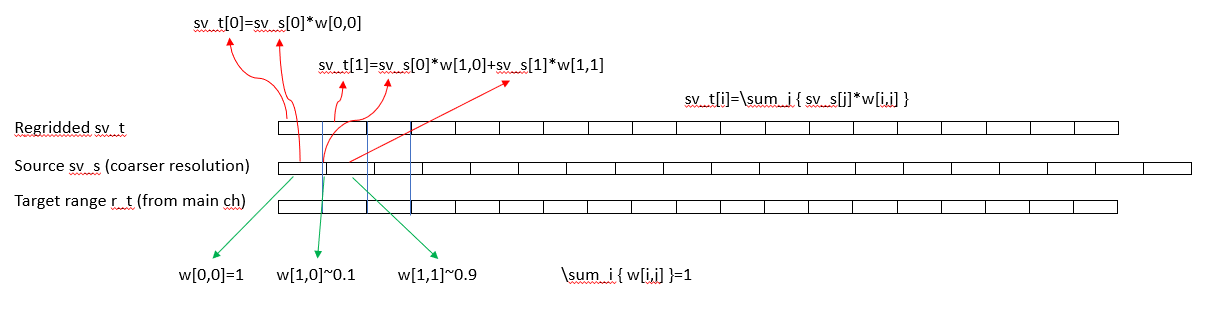
For regridding in range, a first order conservative regridding should be used. This preserve the echo energy when integrating across range. We tested the following approach. For each ping there is a source range vector ‘r_s’, the source sv_s vector, a target range ‘r_t’ coming from the “master” frequency, and the resulting target sv_t ( Figure 11 ). The source range vector can either be of higher or lower resolution than the target range vector. The target range vector is typically the main frequency used for the echo integration, but it can be any of the frequencies. The mapping is a linear mapping between the source and target and the weight matrix is sparse with most weights close to the diagonal. An example can be found here https://github.com/CRIMAC-WP4-Machine-learning/CRIMAC-preprocessing/blob/NOH_pyech/regrid.py , but any mapping that conserve the mass between the grids could be used and standard packages may be used for this purpose.
There are several approaches to grid the data, and each step require more pre-processing with potential data loss. There was a thorough discussion on how much processing could be allowed before passing it onto a ML framework. The idea is that most of these steps can be potentially better handled by the ML framework than ad hoc decision on the pre-processing. The conclusion was to define a set of pre-processing steps, where the first step would be lossless, followed by steps that are near-lossless, e.g. only resample in rare occasions, to more fully gridded version where both time/distance travelled and depth/range a gridded to a uniform grid. If a gridding operation is performed, it should also be labelled in the data. For the latter the resolution may be set similar to the reports that goes into the ICES acoustic data vase, efficiently supporting the whole processing pipeline.
The outcome of this discussion is documented here:
https://github.com/ices-publications/SONAR-netCDF4/issues/33
And in the following pull request:
https://github.com/ices-publications/SONAR-netCDF4/pull/34
3.4.3 - The ICES sonar-netcdf convention
After casting the data into an array/tensor, the convention needs to support storage. To learn more about the different options, we set up some test code for writing NC fields. The echopype package can write both nc and zarr files, but the convention needs to catch up. The objective of this sub task was to go through the steps and write up an np array to .nc to develop the gridded group in the standard.
The test method ek2nc() writes a 3d numpy array to a netcdf4 file. The method takes three parameters:
-
variable : the actual 3d array with dimensions in order (time, range/bins, channels)
-
dims: a list of dimension variables in the same order as indicated for the “variable” parameter above
-
file: the filename as a text string
Gradually the method will be extended to comply with the Sonar-NetCDF standard. Since the parameters to the implemented method do not contain metadata information, this must be supplied manually. After a preliminary comparison between the information content of the EK80 object in Python and the Sonar-NetCDF convention, it seems that part of the data will always have to be provided manually, unless the PyEchoLab package can be updated to draw the information from the raw files. This would be part of a strategy where the ek2nc method receives an EK80 object, possible regridding is done inside the method, and all the meta-information is transferred from the EK80 object to the NetCDF file.
What order should the axis be in? Local in time-space first? Time last since that may cover a full survey? See discussion in this thread: https://github.com/ices-publications/SONAR-netCDF4/issues/33. In theory the ordering of the dimensions, time, range/bins, and beams, can have an impact on I/O performance because a 3D array is essentially a (preferentially contiguous) 1D (chunked) array in memory and on disk. As a result, performance of accessing subsets along one dimension can vary with dimension, because the file pointer may have to jump back and forth if reading along a suboptimal dimension.
Numpy use by default row major ordering of array cells in memory, like C; i.e. C-major ordering), but can also store in column major ordering (like Fortran, Matlab and R; i.e. F-major ordering). NetCDF also uses row-major ordering, implying that there is a 1-1 association in the cell ordering between Python and NetCDF.
for i in ...: for j in ...: for k in ...: A[i][j][k] = .... # efficient in Python, inefficient in Fortran
In NetCDF's row-major ordering the first dimension a of an array A with dimensions (a,b,c) is the slowest and c the fastest changing dimension. This means that, if we want to load entire water column profiles of backscatter but only over limited periods of time, time should be the first and slowest dimension (in NetCDF terms also called the record dimension). In classical NetCDF (< 3.6) it was mandatory to put this dimension FIRST.
As to which dimension to choose as second, several considerations need to be taken into account.
-
We may cut off part of the profiles that are under a bottom (for instance if a technician is not paying attention during a survey to adjust the transducer ranges over the continental slope). But to do this we have to look at the data first, which implies that we have to load it (or at least one channel). Subsetting along the beam range is in theory quicker if the beam dimension is chosen as the second dimension.
-
We may decide to use only a subset of channels, in which case we can optimize by putting the channel dimension second.
NetCDF uses chunking. Chunks are smaller units of data that can be at random position in a file and that are optimally accessed. Chunking and chunk caching (~ keeping in memory what is regularly used) are features that are by default taken care of by the NetCDF software layer. Chunk size and layout are determined based on the sizes of the fixed dimensions. This makes a decision on the order of the fixed dimensions less urgent. Optimizing chunking for one type of data access is likely to worsen other types of data access. It may also be worthwhile to consider how the data is used in Python.
In this early stage, the implemented function (github) to write an Numpy array to NetCDF requires the unlimited time dimension to be the first, followed by the range/bin dimension, and the channel dimension.
This needs to be aligned with the data standard.
3.4.4 - Fitting EK80 FM data into the gridded structure
The EK80 raw format stores the raw sample data and allows for more processing. The volume backscattering (or Target Strength) compressed over the operational frequency band at each sample can directly follow the proposed structure of EK60 and EK80 CW.
Volume backscattering (or Target Strength) as a function of frequency (frequency index m) requires additional processing, which is not implemented in echoPype. There are also choices made in the processing that have implications (e.g. length/distance of the FFT window). There are a few possibilities to do this.
-
Converting complex data to sv at centre frequency. This is the simplest option, but it does not take advantage of the extra information in the FM data.
-
Converting complex data to sv at multiple frequency bands. This will extract some of the information in the FM data. The result will look as multiple CW frequencies.
-
Converting complex data to continuous sv(f) (or TS(f)) for ranges of samples. But how should the sample ranges be chosen? This could be done for the samples of a single target (fish), or for the depth range of a school.
-
Using the complex sample data directly in the machine learning step. This could also need all the meta-data used for converting to sv, such as pulse duration, transmit power, calibration data, etc.
This question has been raised for ICES, and the discussion can be found here: https://github.com/ices-publications/SONAR-netCDF4/issues/33#issuecomment-745347642
3.4.5 - Converting NC data to memmaps
The echogram class used in the COGMAR project currently relies on the data being stored as numpy memory maps (see section above). This file format allows the user to read only a small part of a large file, without loading the entire array into memory. The netCDF files will need to be interfaced with the echogram class for the COGMAR pipeline to work.
One option is to convert the data from the netCDF to the COGMAR files. A conversion script can easily be created, using the netCDF4 python package, to read the relevant parts of the netCDF files. This will be a simple first solution to extend the pipeline to other surveys being prepared in the netCDF format.
Another option is to rewrite the echogram class and read the netCDF files directly during training. The echogram class is used to repeatedly fetch small subsets (contiguous ping-range patches) of the echogram for the training of a neural network. The netCDF allows subsetting, but the access speed must be evaluated. To avoid slowing down the training, this task needs to run quickly and be memory efficient. Instead of using the netCDF4 python package, the xarray python package seems to be a better option. This option needs to be tested.
Being integrated with Dask, xarray allows computations on a dataset similarly to a numpy memory map, i.e. there is no need to load the entire array into memory in order to access a subset. The array is divided into smaller chunks, where the shape of the chunks is determined by the user. Selected chunks may be loaded into memory in an explicit conversion step. The chunk shape may be selected so that it matches the patch size currently used in the training of the neural network. The patch selection could be rewritten so that only one chunk is loaded when selecting a patch. Alternatively, the patch selection may be kept as is, as loading multiple chunks into memory should not affect the performance much.
An example of Xarray-way of chunked read a NetCDF4 file can be found here: https://github.com/iambaim/crimac-hackathon/blob/main/nctomap.ipynb (notebook) or https://github.com/iambaim/crimac-hackathon/blob/main/nctomap.py (Python code).
4 - Concluding remarks
There are several tasks that needs attention on a shorter and longer time scale:
- A data convention for preprocessing and gridding the acoustic data is needed
- Regridding should be avoided if possible, but is needed in cases where pulse lengths are set different (CW)
- The convention for preprocessing FM data needs to be developed
- The preprocessed data should be directly usable by the deep learning frameworks
- There is a need to address data provenance throughout the processing pipelines
- There is a need to develop a standard for annotations
- Existing ML models should be interfaced to the the standard
- Build further processing algorithms should be built on to of the standard
Both the COGMAR project and CRIMAC will follow up on these recommendations, and contribute to the international processes aiming at developing a common community standard for these instruments: https://github.com/ices-publications/SONAR-netCDF4
5 - References
Brautaset, O., Waldeland, A. U., Johnsen, E., Malde, K., Eikvil, L., Salberg, A.-B., and Handegard, N. O. 2020. Acoustic classification in multifrequency echosounder data using deep convolutional neural networks. ICES Journal of Marine Science, 77: 1391–1400.
Korneliussen, R. (Ed). 2018. Acoustic target classification. ICES Cooperative Research Report, No. 344: 104pp.