[Text]
Fisheries survey in the offshore wind power field Hywind Tampen before development
Rapportserie:
Toktrapport 2022-15
ISSN: 1503-6294
Publisert: 09.01.2023
Oppdatert: 24.08.2024
Toktnr: 2022005
Prosjektnr: 15864
Oppdragsgiver(e): Equinor
Referanse: Kari Mette Murvoll
Godkjent av:
Forskningsdirektør(er):
Geir Lasse Taranger
Programleder(e):
Henning Wehde
English summary
1 - Introduction
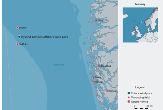
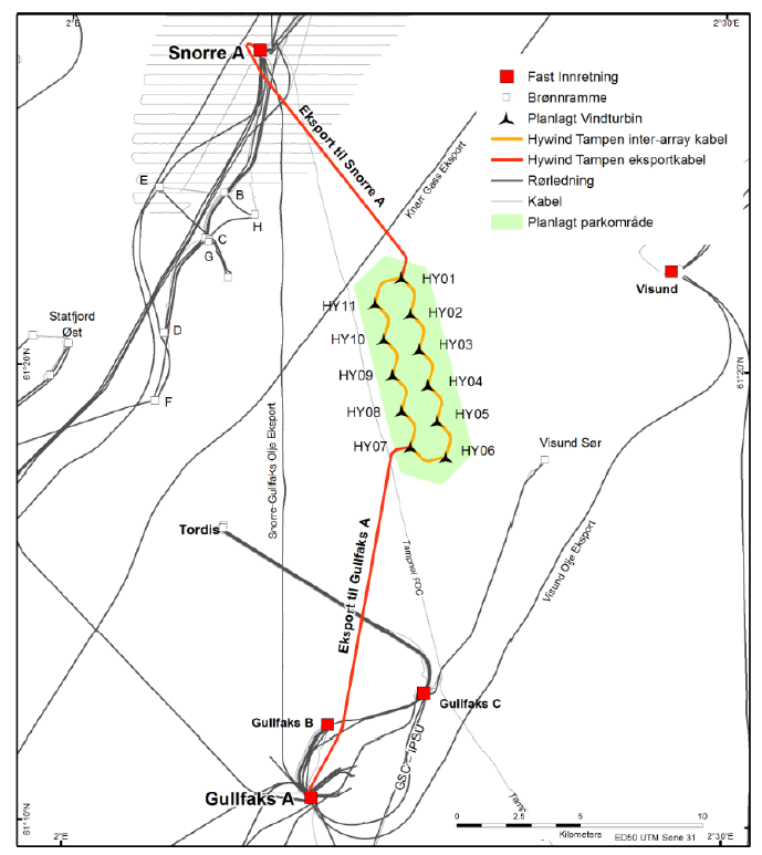
The purpose of the cruise was to carry out a fish capture experiment in the area where a floating windfarm will be built to supply the oil and gas installations with renewable energy. The windfarm is located on the south side of the fishing ground Tampenbanken on the slope down to the Norwegian Trench, (See map figure 1). The windfarm is located at depths between 290 and 300 meters. The wind turbines planned in the park will be floating and must be anchored to the bottom with suction anchors. The windfarm will supply electricity to the oil platforms at Gullfaks and Snorre (Equinor 2019).
2 - Methods
This cruise was conducted between March 24 at 12:30 and April 2 at 08:00 2022 with a chartered fishing vessel. The weather conditions during the cruise were relatively good for the season with winds up to 12-15 m / s and maximum wave height of 2.5 -3 meters. Current conditions were favorable throughout the period, with current speeds of 0.3 to 0.5 knots throughout the water column. The dominant current direction was Northeast - Southeast. Water temperature was around 8 ֯ C during the cruise period.
| Name | Affiliation | Role |
| Karen de Jong | Institute of Marine Research | Cruise leader |
| Kate McQueen | Institute of Marine Research | Researcher |
| Nils-Roar Hareide | Institute of Marine Research / Runde Miljøsenter | Researcher |
| August Feldskår | Nesefisk AS | Captain |
| 5 | Nesefisk AS | Crew |
2.1 - Vessel details
The fishing vessel Nesejenta (AG-1-LS) conducts commercial fishing for demersal fish in the North Sea, the Norwegian coast and the Barents Sea. The vessel was equipped for fishing with gillnets and Danish seine. Nesejenta was built in 2020 with a length of 35.3 m, width 9.10 m and a gross tonnage of 499 tons. Engine power 998 HP, Load capacity: 80 tons
The vessel was equipped with a current meter and fish finding equipment including a Furuno FCD 1900 echosounder and a Wassp multibeam sonar. In addition, the vessel had an Olex map machine that was used for navigation and planning of fishing operations.
2.2 - Fishing gear
We used 5 links of 80 nets, of these, there were 20 cod nets and 60 saithe nets. Each link had a length of 28 meters. Mesh size of the saithe nets: 74 mm half stitch, Cod nets 90-93 mm (half mesh). A maximum of 5 links could be set each day.
2.3 - Experimental design
A gradient approach was chosen with stations at different distances from the wind farm, because a before-after gradient (distance-based) approach has been identified as one of the most powerful methods to assess ecological effects of offshore wind farms in the field (Methratta 2021). We identified 8 stations, at increasing distance from the planned location of the windfarm (Table 1). Each day 3-5 links were distributed over these stations.
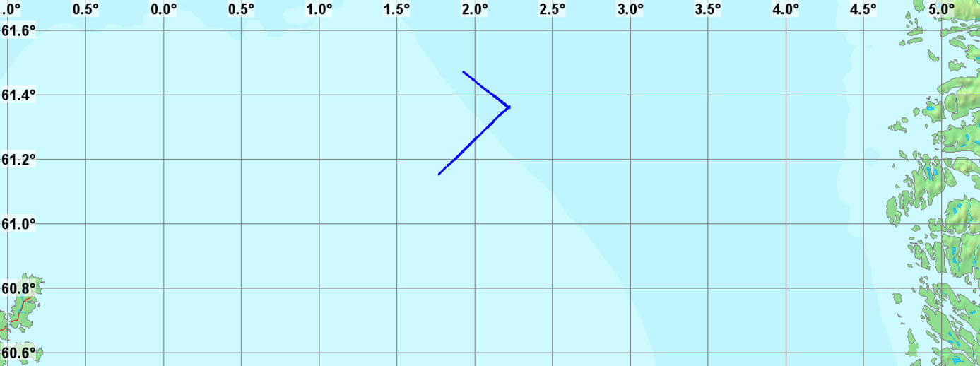
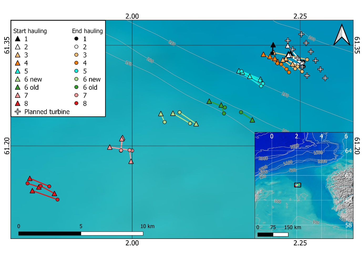 Figure 3: The hauling positions of gillnets, with station number denoted by colour. Start and stop positions of each haul are connected by a line. Depth contours (© Kartverket) and planned positions of turbines are shown. Inset map shows study area in relation to the southern part of the Norwegian coast/the Norwegian Trench (© GEBCO).
The fishing was done with gillnets by professional fishermen using the fishing vessel’s own quota, and the fish were sold afterwards. A total of 34 catches were conducted, with 3-4 replicate catches per station (Table 2). Station 6 was lost twice, likely due to bottom conditions and the steeper slope. We therefore created a new station 6 during the survey (Figure 3, Table 2). Data from the original Station 6 are shown in the figures but were not included in statistical analyses. All fish were brought on board and sampling followed standard procedures for the Reference Fleet in Norway: taking samples for the first twenty fish for each species in each catch (Mjanger et al. 2022). Fish were measured to the nearest cm below and weighed to the nearest gram up to a maximum of twenty fish per catch. For hyse/haddock, lange/ling, lysing/hake, sei/saithe and torsk/cod, we also took stomach samples of the first twenty fish at each location (Table 3). Some fish had inverted stomachs due to the pressure change during hauling, these stomachs were not collected. This phenomenon was especially common in ling, but due to the high abundance of ling overall, most stomach samples were from ling (114 of 362). Because we only caught 34 haddock in total, we did not include these stomach samples in further analyses, resulting in a total of 335 stomach samples from 4 species. Especially in the catches close to the windfarm, fish were eaten by sea lice while caught in the nets. In such cases a measurement of length was often still possible, but the weight was not measured.
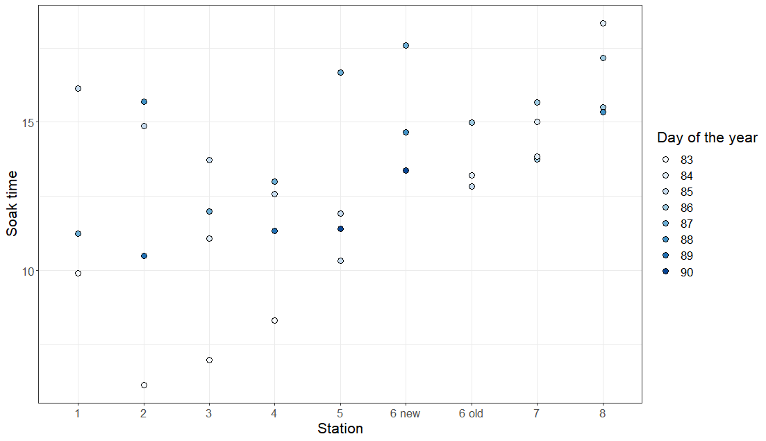
Weather conditions and the wish to limit soak time in the area with a lot of sea lice (station 1-3) prevented a fully randomized design. As a result, there was a significant, positive relationship between soak time and distance to turbine (p < 0.001, R2 = 0.28) This pattern seems to be driven by three sets with especially short soak times close to the windfarm (Figure 4). In the analyses, we corrected species richness and abundance measures for soak time (see statistical approach).
2.4 - Statistical Approach
While the figures shown in this report represent the data per station, the statistical analyses were done using linear models with the distance to the windfarm site as a continuous explanatory variable. This distance was calculated from the midpoint of each gillnet to turbine 9 (61.33N, 2.25E) (See table 2). To separately assess the effect of the distance to the windfarm site and the effect of depth on species richness the data were split into two depth categories (deep: station 1-5 and shallow: station 6-8). Poisson GLMs were conducted to assess whether species richness varied with distance from the windfarm site within these depth categories. In addition, a model was fitted to test for a difference in species richness between the two depth categories. Soak time in hours was included as an offset in all models.
The most abundant species caught, which are also of commercial interest, were ling, hake, saithe and cod. To assess how abundance of these key species varied along the transect, the same modelling approach as described for species richness was used. The proportion of spawning fish in the samples of key species was compared between depth strata and then between stations using a similar method, but this time using a binomial GLM. Maturity data were available for ling, cod, hake and saithe. Some maturity data were collected from haddock, but sample sizes were too small (n = 27; Table 3) to conduct analysis.
| Station | Serial Nr. | Repl. nr. | Date set | Time set | Soak time | Latitude (start) | Longitude (start) | Latitude (end) | Longitude (end) | Distance from planned windfarm | Fishing depth (average) |
| 1 | 57908 | 1 | 25.03.2022 | 23:50 | 9.92 | 61.33750 | 2.23250 | 61.32533 | 2.25500 | 0.13 | 282.75 |
| 57934 | 2 | 27.03.2022 | 23:32 | 16.13 | 61.33833 | 2.23567 | 61.31833 | 2.25533 | 0.28 | 286.00 | |
| 57946 | 3 | 29.03.2022 | 22:00 | 11.25 | 61.35083 | 2.20983 | 61.33817 | 2.20833 | 2.49 | 286.00 | |
| 2 | 57901 | 1 | 25.03.2022 | 03:45 | 6.15 | 61.33500 | 2.23500 | 61.32350 | 2.25383 | 0.19 | 282.00 |
| 57932 | 2 | 27.03.2022 | 23:13 | 14.87 | 61.32967 | 2.22800 | 61.32100 | 2.24667 | 0.76 | 284.25 | |
| 57960 | 3 | 30.03.2022 | 23:58 | 15.70 | 61.34950 | 2.23150 | 61.33000 | 2.24783 | 1.05 | 284.00 | |
| 57961 | 4 | 31.03.2022 | 22:40 | 10.50 | 61.33550 | 2.23267 | 61.32233 | 2.25267 | 0.27 | 286.00 | |
| 3 | 57903 | 1 | 25.03.2022 | 04:15 | 7.00 | 61.33033 | 2.22883 | 61.31833 | 2.24617 | 0.85 | 278.00 |
| 57910 | 2 | 26.03.2022 | 00:10 | 11.08 | 61.32217 | 2.23867 | 61.31083 | 2.25283 | 1.59 | 280.00 | |
| 57929 | 3 | 27.03.2022 | 22:56 | 13.73 | 61.32833 | 2.22433 | 61.31500 | 2.24250 | 1.22 | 281.75 | |
| 57947 | 4 | 29.03.2022 | 22:20 | 12.00 | 61.33933 | 2.21050 | 61.32867 | 2. 26033 | 0.66 | 282.50 | |
| 4 | 57905 | 1 | 25.03.2022 | 04:25 | 8.33 | 61.32583 | 2.21667 | 61.31450 | 2.22967 | 1.70 | 274.00 |
| 57927 | 2 | 27.03.2022 | 22:40 | 12.58 | 61.33050 | 2.21233 | 61.30967 | 2.23333 | 1.72 | 279.00 | |
| 57949 | 3 | 29.03.2022 | 22:40 | 13.00 | 61.33667 | 2.19533 | 61.32300 | 2. 21617 | 2.15 | 279.00 | |
| 57963 | 4 | 31.03.2022 | 23:10 | 11.33 | 61.33333 | 2.20500 | 61.32167 | 2.22183 | 1.77 | 280.00 | |
| 5 | 57917 | 1 | 27.03.2022 | 00:40 | 10.33 | 61.30383 | 2.17500 | 61.29283 | 2.19450 | 4.87 | 252.50 |
| 57926 | 2 | 27.03.2022 | 22:15 | 11.92 | 61.31000 | 2.16383 | 61.29717 | 2.19017 | 4.77 | 256.00 | |
| 57952 | 3 | 29.03.2022 | 23:10 | 16.67 | 61.31200 | 2.15883 | 61.28917 | 2.19183 | 5.05 | 252.50 | |
| 57966 | 4 | 01.04.2022 | 00:05 | 11.42 | 61.29950 | 2.19100 | 61.31117 | 2.16267 | 4.65 | 256.00 | |
| 6_old | 57912 | 1 | 26.03.2022 | 00:35 | 13.22 | 61.26100 | 2.13250 | 61.24833 | 2.13667 | 10.36 | 166.50 |
| 57919 | 2 | 27.03.2022 | 00:10 | 12.83 | 61.26667 | 2.11467 | 61.25733 | 2.13800 | 9.98 | 184.50 | |
| 57935 | 3 | 28.03.2022 | 19:16 | 14.98 | 61.23883 | 2.17883 | 61.25017 | 2.16200 | 10.42 | 192.00 | |
| 6_new | 57954 | 1 | 29.03.2022 | 23:45 | 17.58 | 61.24867 | 2.06067 | 61.23350 | 2.08617 | 13.60 | 136.00 |
| 57958 | 2 | 30.03.2022 | 22:40 | 14.67 | 61.24817 | 2.04267 | 61.23550 | 2.04833 | 14.59 | 138.00 | |
| 57968 | 3 | 01.04.2022 | 00:22 | 13.38 | 61.23300 | 2.09517 | 61.25000 | 2.07050 | 13.23 | 138.00 | |
| 7 | 57914 | 1 | 26.03.2022 | 01:25 | 13.83 | 61.21250 | 1.98567 | 61.19283 | 1.98333 | 19.98 | 141.00 |
| 57921 | 2 | 26.03.2022 | 23:40 | 15.00 | 61.19833 | 1.96667 | 61.19300 | 2.00000 | 20.59 | 137.00 | |
| 57938 | 3 | 28.03.2022 | 21:55 | 13.75 | 61.17717 | 1.99833 | 61.19367 | 1.99617 | 20.96 | 139.00 | |
| 57940 | 4 | 28.03.2022 | 21:30 | 15.67 | 61.21067 | 1.98450 | 61.19333 | 1.98350 | 20.05 | 140.00 | |
| 8 | 57924 | 1 | 26.03.2022 | 22:00 | 18.33 | 61.15167 | 1.84767 | 61.13967 | 1.87667 | 34.65 | 137.00 |
| 57942 | 2 | 28.03.2022 | 23:00 | 15.50 | 61.13333 | 1.85150 | 61.12000 | 1.88900 | 29.11 | 137.00 | |
| 57944 | 3 | 28.03.2022 | 22:40 | 17.17 | 61.12917 | 1.88433 | 61.14033 | 1.86383 | 30.36 | 138.50 | |
| 57956 | 4 | 30.03.2022 | 20:10 | 15.33 | 61.13883 | 1.86117 | 61.14417 | 1.84433 | 29.55 | 138.00 |
| Species: Norwegian name | Species: English name | Species: Scientific name | Total caught | Nr. of samples: Length | Nr. of samples: Weight | Nr. of samples: Maturity | Nr. of stomach samples |
| breiflabb | European angler | Lophius piscatorius | 20 | 20 | 16 | ||
| brosme | Tusk | Brosme brosme | 15 | 15 | 14 | ||
| gapeflyndre | American plaice | Hippoglossoides platessoides | 8 | 8 | 7 | ||
| gjøkskate | Leucoraja naevus | 1 | 1 | 1 | |||
| glassvar | Megrim | Lepidorhombus whiffiagonis | 9 | 9 | 9 | ||
| havmus | Rabbit fish | Chimaera monstrosa | 58 | 47 | 39 | ||
| hvitting | whiting | Merlangius merlangus | 141 | 113 | 111 | ||
| hyse | Atlantic haddock | Melanogrammus aeglefinus | 34 | 34 | 33 | 32 | 27 |
| hågjel | Blackmouth catshark | Galeus melastomus | 35 | 30 | 25 | ||
| kloskate | Thorny skate | Amblyraja radiata | 3 | 3 | 3 | ||
| knurr | Grey gurnard | Eutrigla gurnardus | 3 | 3 | 3 | ||
| kolmule | Blue whiting | Micromesistius poutassou | 41 | 41 | 37 | ||
| kveite | Atlantic halibut | Hippoglossus hippoglossus | 3 | 3 | 2 | ||
| lange | Common ling | Molva molva | 589 | 326 | 299 | 307 | 114 |
| lyr | Atlantic pollock | Pollachius pollachius | 69 | 51 | 51 | ||
| lysing | European hake | Merluccius merluccius | 84 | 84 | 80 | 79 | 46 |
| makrell | Atlantic mackerel | Scomber scombrus | 47 | 45 | 44 | ||
| nebbskate | Shagreen skate | Leucoraja fullonica | 3 | 3 | 2 | ||
| pigghå | Spiny dogfish | Squalus acanthias | 8 | 8 | 7 | ||
| sei | Saithe | Pollachius virens | 158 | 158 | 140 | 141 | 96 |
| sild | Atlantic herring | Clupea harengus | 1 | 1 | 1 | ||
| skjellbrosme | - | Phycis blennoides | 2 | 2 | 2 | ||
| smørflyndre | Righteye flounder | Glyptocephalus cynoglossus | 1 | 1 | 1 | ||
| storskate | Common skate | Dipturus inter-medius (D. batis) | 6 | 6 | 7 | ||
| svartflabb | Blackbellied angler | Lophius budegassa | 1 | 1 | 1 | ||
| torsk | Atlantic cod | Gadus morhua | 215 | 187 | 186 | 186 | 79 |
| vanlig uer | Atlantic redfish | Sebastes norvegicus | 1 | 1 | 1 | ||
| vassild | Greater argentine | Argentina silus | 1 | 1 | 1 | ||
| Total | 1557 | 1202 | 1123 | 745 | 362 |
2.5 - Acoustic data collection
Two acoustic transects were repeated several times during the survey (Table 4). One transect was in a southwest direction from the planned windfarm (SW) and the other in a northwest direction (NW) (Figure 5). The SW transect was 20 nm and covered the same area as the gill net stations (Figure 3). The water depth along the SW transect varied from about 300 m closest to windfarm to 106 m at the furthest point and was covered 4 times, twice in each direction. The NW transect was 10 nm long and covered twice in each direction. The depth on the NW transect was constant at about 300 m. All acoustic transect data were collected between midnight and 05:00 UTC (Table 4). The vessel speed during the transects varied between 5 and 6 kts. Acoustic data were collected using the Wassp multibeam sonar. The sonar has a fan of beams arranged perpendicular to the vessel’s alongship axis, and five inspection beams, all operating at 160 kHz. All beam data were stored to computer, but only the inspection beam that pointed vertically down was used in the analyses, as this most closely matches a conventional echosounder. The angle of this beam was set to 10 degrees, the sonar ping rate was approximately 1 Hz and the ping duration was 1 ms. The amplitude response of the sonar was not calibrated.
The Wassp data files were converted to Simrad EK60 format to enable processing in IMR’s acoustic survey software (LSSS). The Korona module in LSSS was used to remove noise from the acoustic data. Acoustic backscatter data were divided into three depth layers; a surface layer at 5 – 25 m, a bottom layer from 25 m above the seabed to 5 m above the seabed, and a mid-layer covering the ranges between the surface and seabed layers. The 25th, 50th and 75th quantiles of volume backscattering strength (Sv, re 1m-1 , dB) by ping and within each depth layer (surface, mid and bottom) were calculated. The results are presented as running median values over 11 pings. (~10 s). In addition, a more detailed scrutiny of the data (5 nm steps) was made to identify single targets and aggregations of fish.
| Date | Transect | Start Lat (N) | Start Lon (E) | End Lat (N) | End Lon (E) | Start time (UTC) | End time (UTC) |
| 26.03.2022 | Station 8 to 1 (SW1) | 61° 10' | 1° 49' | 61° 22' | 2° 13' | 02:08 | 04:56 |
| 27.03.2022 | Station 1 to 8 (SW2) | 61° 13' | 2° 14' | 61° 11' | 1° 50' | 03:04 | 05:49 |
| 27.03.2022 | Station 1 to northwest (NW1) | 61° 22' | 2° 13' | 61° 28' | 1° 56' | 22:41 | 00:42 |
| 28.03.2022 | Northwest to station 1 (NW2) | 61° 28' | 1° 56' | 61° 22' | 2° 14' | 00:42 | 02:31 |
| 29.03.2022 | Station 8 to 1 (SW3) | 61° 11' | 1° 50' | 61° 22' | 2° 13' | 00:30 | 03:07 |
| 30.03.2022 | Station 1 to northwest (NW3) | 61° 22' | 2° 13' | 61° 28' | 1° 56' | 00:56 | 02:36 |
| 30.03.2022 | Northwest to station 2 (NW4) | 61° 28' | 1° 56' | 61° 22' | 2° 13' | 02:36 | 04:12 |
| 30.01.1900 | Station 1 to 8 (SW4) | 61° 21' | 2° 13' | 61° 11' | 1° 45' | 23:33 | 01:59 |
2.6 - eDNA collection
Environmental DNA (eDNA) can be collected from water samples to assess which species were in the area, due to animals excreting or losing DNA to the surrounding water. Such methods, however, have not yet been fully developed for the marine environment (Stoeckle et al. 2021). During this cruise we collected water samples at three different distances from the wind farm site to test whether they would give similar results as the catches, and whether they would provide extra information about additional species. Samples were taken at station 1 (at 5 m depth and close to the bottom at 270 m), at station 3 (at 5 m) and at station 8 (close to the bottom at 135 m). There were taken three replicates of surface and two replicates of the bottom water samples at the station 1. At stations 3 and 8 only one sample was taken. The samples were filtered with an eDNA kit provided by NINA (www.nina.no/miljo-DNA/miljo-DNA-i-vann) including a battery-powered peristaltic pump (Vampire sampler, Bürkle GmbH, Bad Bellingen, Germany), a closed filter system with two filters (5.0 µm glass fiber filter and 0.8 µm polyethene sulfone filter, NatureMetrics, Guildford, United Kingdom) and buffer ATL (Qiagen GmbH, Hilden, Germany) to store the filters. The filters were sent to NINA for analyses. There, DNA was extracted using the Nucleospin Plant II Midi kit (Macherey-Nagel GmbH, Düren, Germany), and amplified in PCR reactions using fish-specific mitochondrial 12S rRNA gene primers MiFish-U-F and MiFish-U-R (Miya et al. 2015). The amplicons will be paired-end sequenced (2x150 bp) using Illumina NovaSeq 6000 machine. An updated to this report will be provided when the samples are analysed.
3 - Observations
3.1 - Observations of other fishing activity in the area.
Two Norwegian vessels fished in the survey area or near it. It was Sjøvik and Utvær who fished with bottom trawls after clearing at about 275-300 meters. Nanna Cecilie from Denmark used Danish seine and caught 16 tons in four days. The Danish seine fishery was conducted at 275-315 meters at the edge of the Norwegian Trench east of the Statfjord field and the Gullfaks field. Boy Andrew from Scotland used Danish Seine in the same area as Nanna Cecilie.
3.2 - Observations of seabirds
A good number of seabirds gathered around the vessel and grazed on fish hatcheries that were thrown overboard. No attempt was made to count the number of birds. Several photos were taken and the species of seabirds observed in the area were registered. The most numerous species was the Havhest (Fulmar, Fulmarus glacialis ) followed by the Havsule (Gannet, Morus bassanus ). These two species were by far the most numerous. In addition, some Krykkje (Kittiwake, Rissa tridactyla ) and some Svartbak (black-backed gulls, Larus marinus ) were observed.
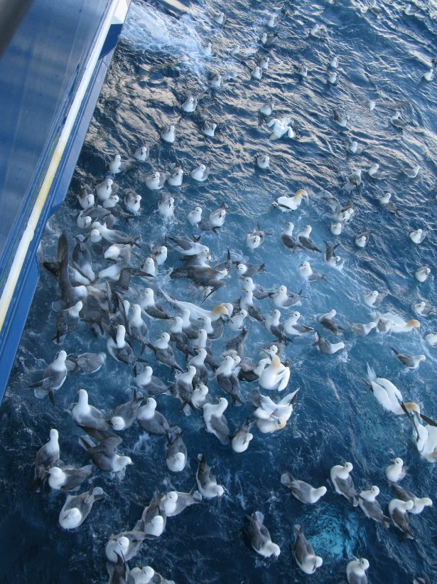
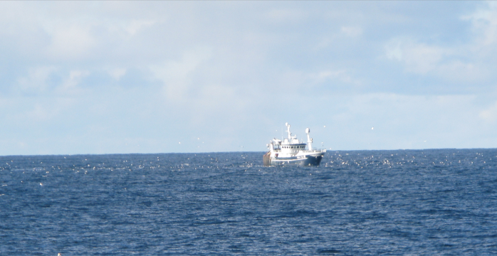 Figure 6. A. Seabirds feeding on fish waste alongside the fishing vessel. B. Seabirds around the fishing vessel. Picture: Nils Roar Hareide.
4 - Experimental results
4.1 - Gill net catches
4.1.1 - Does species richness vary with distance from the planned windfarm?
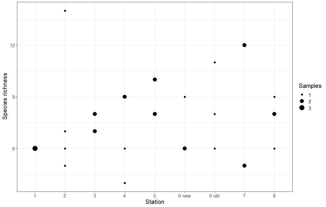
There was no significant relationship between species richness and distance to the windfarm site, within depth categories (shallow: p = 0.91, deep: p=0.22), and no significant difference in species richness between depth categories (p = 0.17; Figure 7).
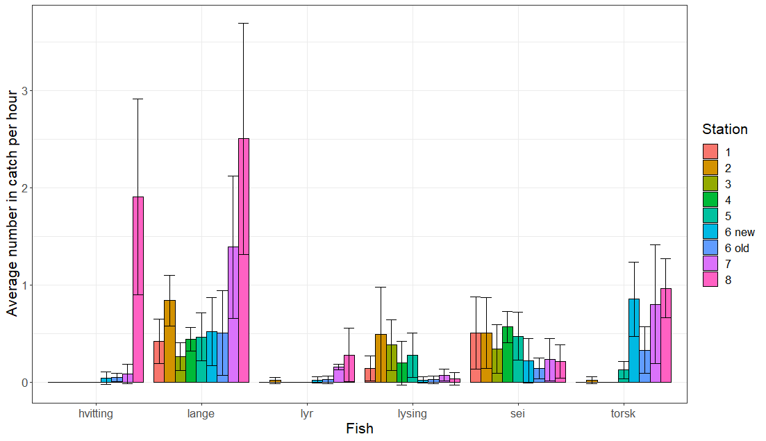
4.1.2 - Does abundance of key species vary with distance from the planned windfarm?
The most abundant species caught, which are also of commercial interest, were ling, hake, saithe and cod. Whiting, ling, pollock and cod were mainly found further outside the windfarm site, while saithe and hake were found closer to the windfarm site (Figure 8). This corresponds to previous data from IMR on spawning areas, as well as catch data from the Norwegian Fisheries Directorate. For most of the abundant species, abundance was related to depth. For cod and ling, there were significantly higher abundances in the shallow region than in the deep region (cod: p < 0.001; ling: p < 0.001). For hake and saithe, on the other hand, there were significantly higher abundances in the deep region than the shallow region (hake: p = 0.004; saithe: p = 0.006). For whiting, 0 whiting were caught in the deep region, and 137 were caught in the shallow region. However, nearly all whiting were caught at a single sampling station (station 8, n = 130), preventing statistical analyses.
Within depth categories, there was some variation in abundances according to distance from Hywind Tampen. For cod, there was no variation in abundance with distance from Hywind Tampen in the shallow region (p = 0.5), but there was an increase in abundance with distance from Hywind Tampen in the deep region (p = 0.007). For ling and whiting, there was increasing abundance with distance from the turbine in the shallow region (ling p = 0.01, whiting p = 0.006). There was no relationship with distance in the deep region for ling (p = 0.57), whiting was not found in the deep region. For saithe and hake, there was no relationship with distance at either depth (saithe, shallow: p = 0.8, saithe, deep: p = 0.4, hake, shallow: p = 0.998, hake, deep: p = 0.39).
For elasmobranchs, there were too low numbers caught to statistically assess differences, but Rabbit fish (havmus) and Blackmouth catshark (hågjel) were only found in the deeper waters close to the windfarm site (Figure 9). The numbers for all other species that were caught in relatively low numbers can be found in Figure 9 and 10.
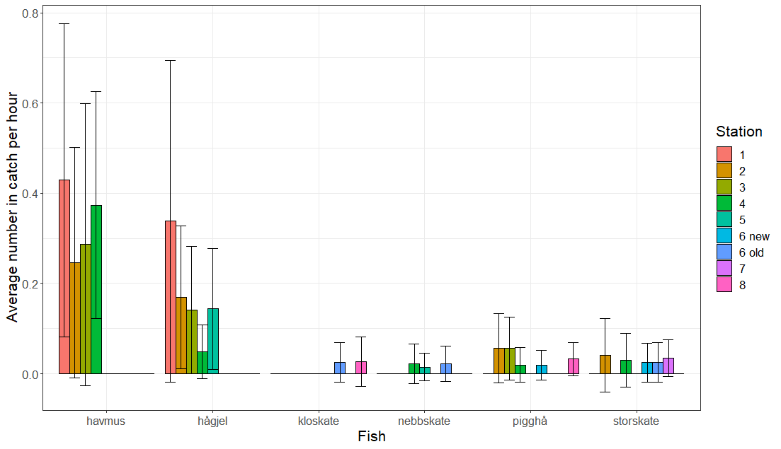
Figure 9: Average number of elasmobranchs caught in gillnets at different distances from the planned location of the windfarm for the six most abundant species. Location 1 was closest to the windfarm site, location 8 was furthest away (Figure 1). Before averaging, the number of fish per catch was divided by soak time to calculate catch per hour. Standard deviations of the means are shown by error bars. See Table 3 for English species names.
4.1.3 - Does maturity of key species vary between stations?
Maturity data were available for ling, cod, hake and saithe (Figure 11). Analysis of the maturity data revealed little variation in proportion of spawning fish between depth categories or distances to the windfarm. For cod, there were maturity data for only 5 fish in the deep region, none of which were spawning, compared to 148 fish in the shallow. Within the shallow region there was no relationship between distance to Hywind Tampen and proportion of spawning cod (p = 0.65).
For ling, there was a significantly higher proportion of spawning fish in the shallow region than the deep (p < 0.001). Within depth categories, there was no significant relationship between proportion spawning and distance to the windfarm site (shallow: p = 0.5, deep: p = 0.2).
For hake, there was again limited sample size, with only 7 observations of maturity data from the shallow region (2 spawning, 5 not spawning). In the deep region, there was no significant relationship between proportion spawning and distance to the windfarm site (p = 0.5).
For saithe, there was no significant difference between depth regions (p = 0.057). Within depth categories there were no significant relationships between proportion spawning and distance to the windfarm site (shallow: p = 0.3, deep: p = 0.3).
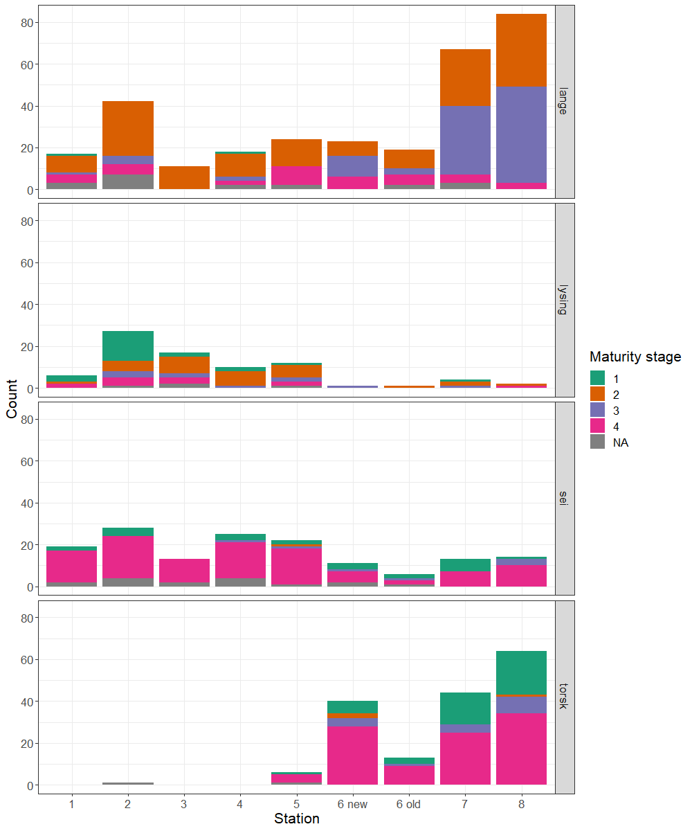 Figure 11. Maturity stage of the four most common species of fish caught in gillnets at different distances from the planned location of the windfarm. Location 1 was closest to the windfarm site, location 8 was furthest away (Figure 1). Maturity stage 1 is immature, 2 is mature, 3 is spawning and 4 is spent: past spawning. See Table 3 for English species names.
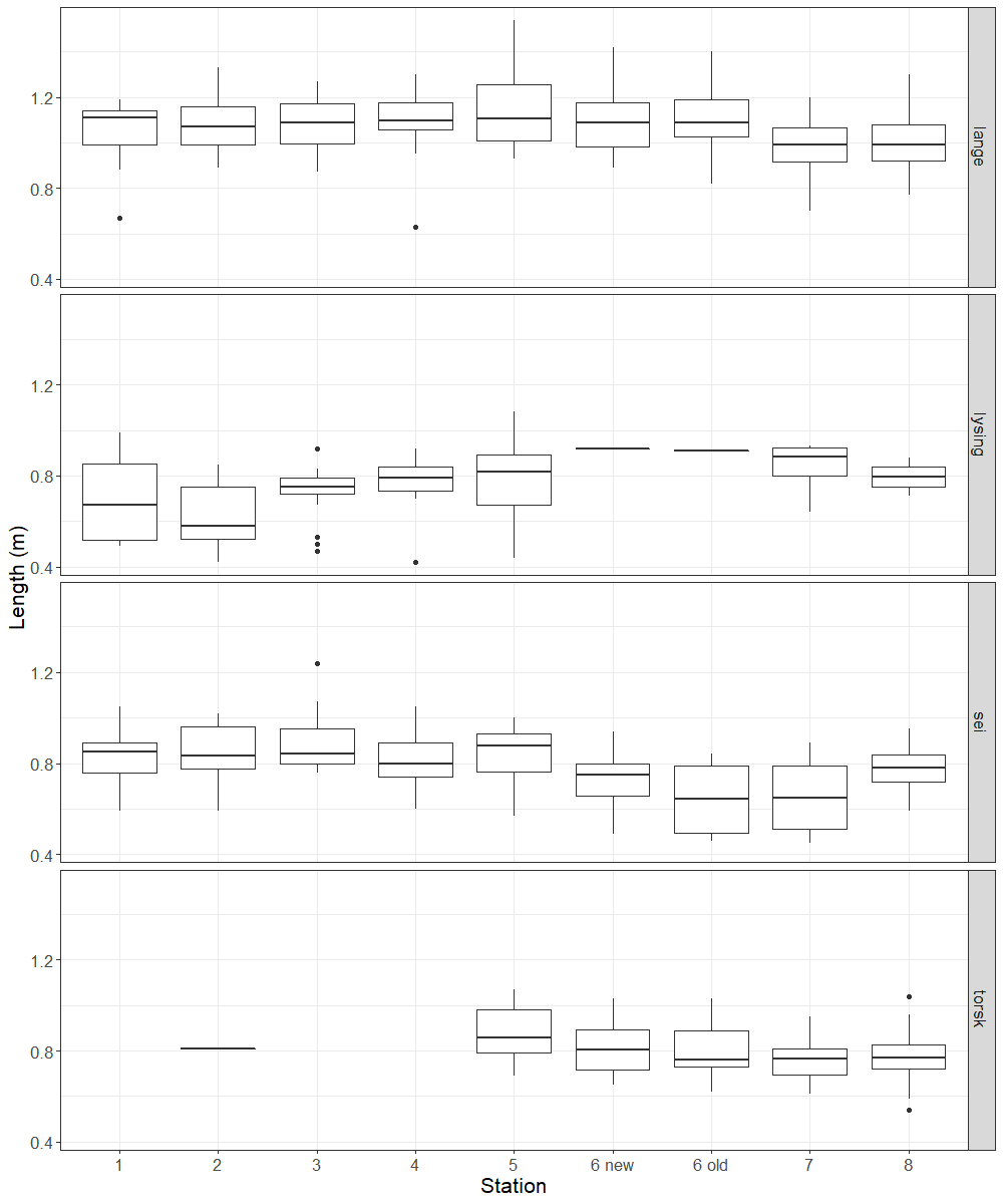
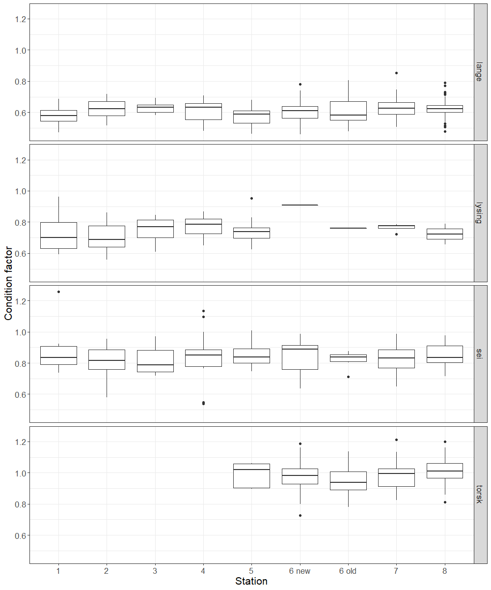
4.1.4 - Size and condition of common fish
Cod in the deep region were significantly larger (length) than cod in the shallow region (p = 0.02). There was no difference in condition factor between depth categories (p = 0.8). There were only 17 cod caught in the deep region. There was no relationship between distance to the turbine and length (p = 0.7) or condition (p = 0.8) in the deep region. In the shallow region, there was no significant relationship between distance to the wind farm and length (p = 0.1), but there was a significant positive relationship between distance to the wind farm and condition (p = 0.01).
Ling in the deep region were larger than ling in the shallower region (p < 0.001). Ling in the shallower region had higher condition factor than ling in the deeper region (p = 0.01). Within the deep region, there was no relationship between length of ling and distance to the wind farm (p = 0.09), but there was a significant, negative relationship between distance to the wind farm and condition factor (p = 0.03). In the shallow region, there was no relationship between length and distance to the wind farm (p = 0.09) or condition factor and distance to the wind farm (p = 0.5).
Hake in the shallow region were larger than hake in the deep region (p = 0.03). There was no difference in condition factor between the depth categories (p = 0.3). Within the deep region, there was a significant, positive relationship between length and distance to the wind farm (p = 0.002), but no relationship between condition factor and distance to wind farm (p=0.3). Only 5 hake were caught in the shallow region, so no further analyses were conducted.
Saithe in the deep region were significantly larger than saithe in the shallow region (p < 0.001). There was no relationship between condition factor and depth category for saithe (p=0.9). In the deep region, there was no significant relationship between distance to turbine and length (p=0.9) or condition factor (p = 0.8). Likewise, in the shallow region, there was no significant relationship between saithe length (p=0.2) or condition factor (p=0.8) and distance to the wind farm.
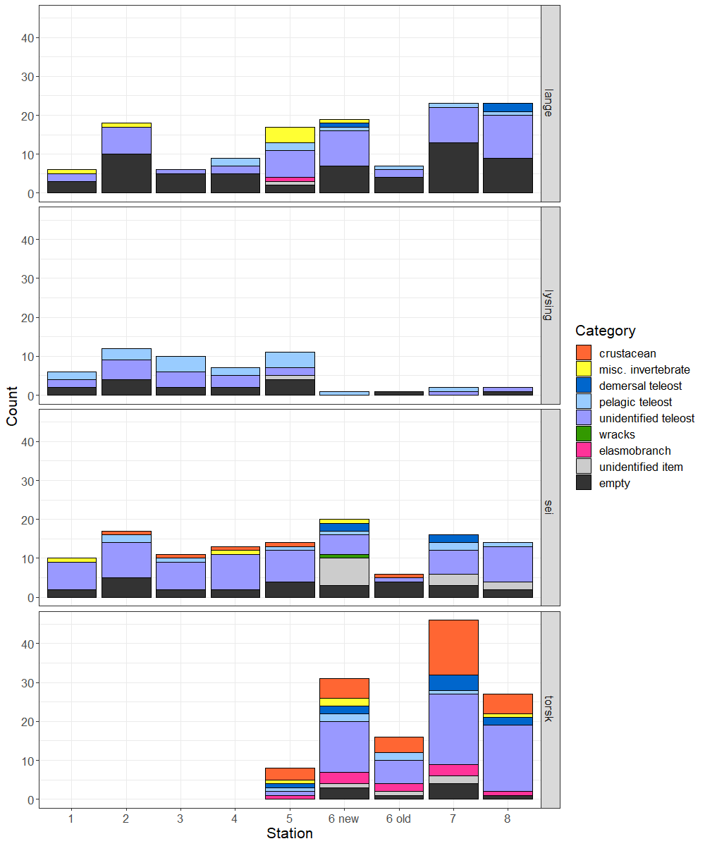
4.1.5 - Stomach content analysis
A variety of prey species were identified from the stomach sampling, though some items could not be identified to species level (Table 5). The stomach content analysis indicated variation in prey between species, as expected, with high proportions of empty stomachs apparent in some species and stations (Figure 14). Mackerel were the most common food item and were found in stomachs at all stations. Mackerel were found in stomachs of hake, saithe, ling and cod.
| Category | Name | n |
| crustacean | crustaceans | 18 |
| deep sea shrimp | 1 | |
| gammarid amphipods | 1 | |
| short-tailed crabs | 2 | |
| shrimps | 3 | |
| squat lobsters | 4 | |
| stone crab | 4 | |
| great spider crab | 2 | |
| krill | 1 | |
| misc. invertebrate | bivalves | 1 |
| brittle stars | 1 | |
| gastropods | 1 | |
| isopods | 9 | |
| squids. octopusses | 2 | |
| demersal teleost | atlantic hookear sculpin | 1 |
| haddock | 3 | |
| long rough dab | 5 | |
| norway pout | 3 | |
| redfishes | 1 | |
| rockfishes | 1 | |
| whiting | 2 | |
| pelagic teleost | atlantic herring | 1 |
| blue whiting | 4 | |
| garfish | 1 | |
| mackerel | 28 | |
| norwegian spring-spawning herring | 5 | |
| unidentified teleost | teleosts | 184 |
| elasmobranch | blackmouthed dogfish | 1 |
| sea mouse | 9 | |
| skates and rayes | 1 | |
| wracks | wracks | 1 |
| unidentified item | unidentified | 18 |
| empty | NA | 110 |
4.2 - Acoustic data
Median acoustic backscatter strengths (Sv, dB re 1 m-1) ranged between -60 and -90 dB and the registrations were relatively similar between replicates. In the southwestern transect (Figure 15 and Figure 17) higher Sv values in the surface layer were registered in the shallower areas further away compared to the deeper waters closer to the windfarm site. On the other hand, in the bottom layer higher Sv values were registered in the deeper waters compared to the shallower water further away from the windfarm site. Sv values in the mid layer were variable and no clear trends related to distance to windfarm or bottom depth were registered.
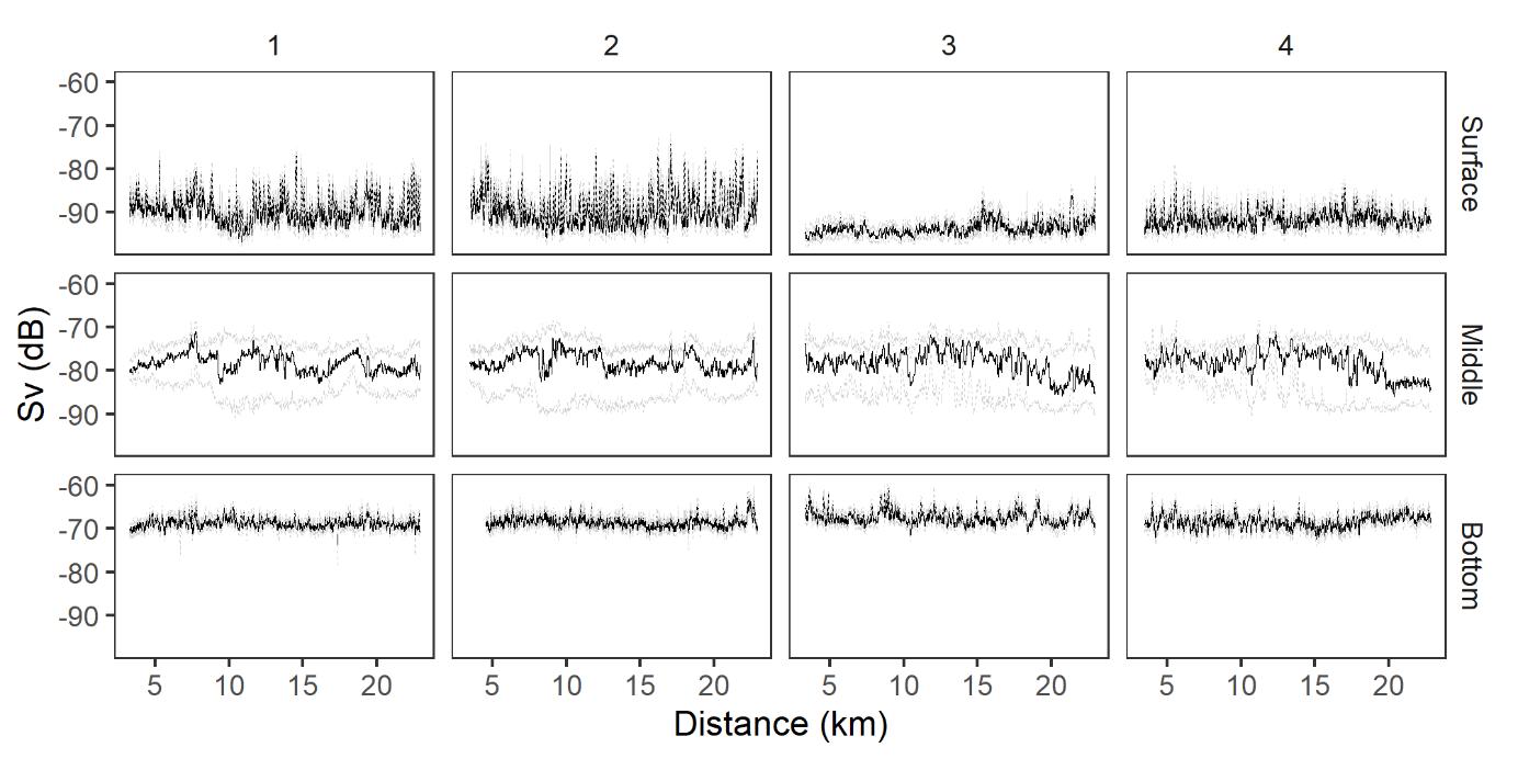
In the northwestern transect no clear trends in Sv values related to distance from windfarm or water depth were registered (Figure 16 and Figure 18). The backscatter was strongest in the bottom layer and weakest in the surface layer.
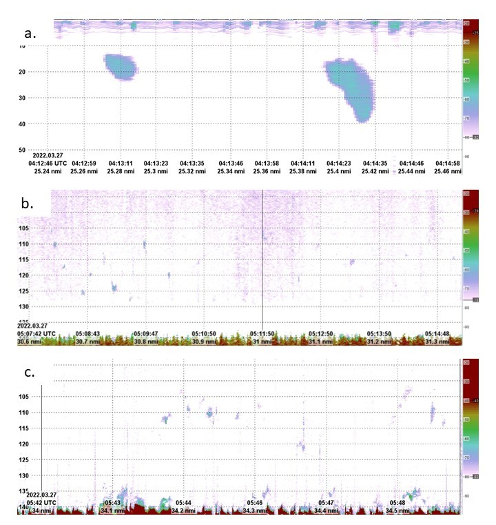
In general, very few fish schools were registered in the acoustic survey. Some slightly denser aggregations of organisms were registered in the southwestern transect where bottom depth was between 140 and 150 m (Figure 19).
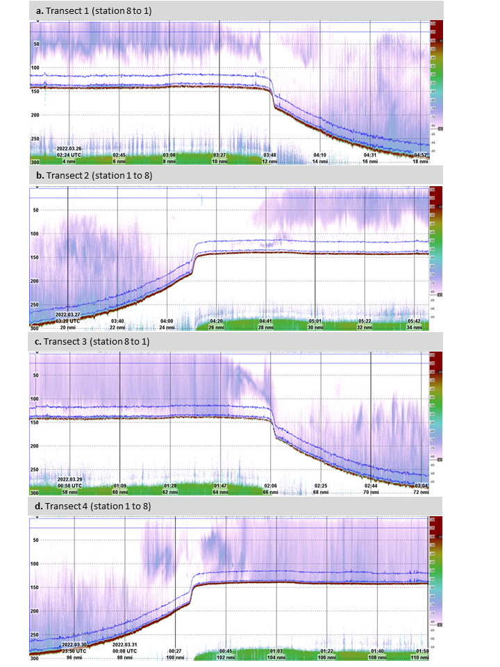
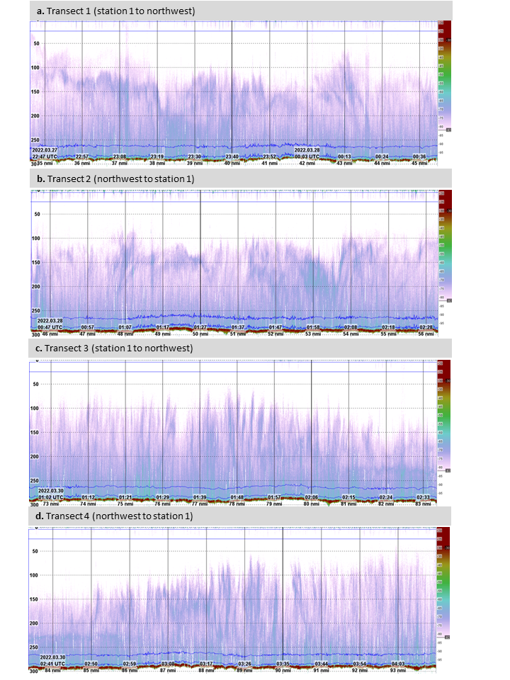
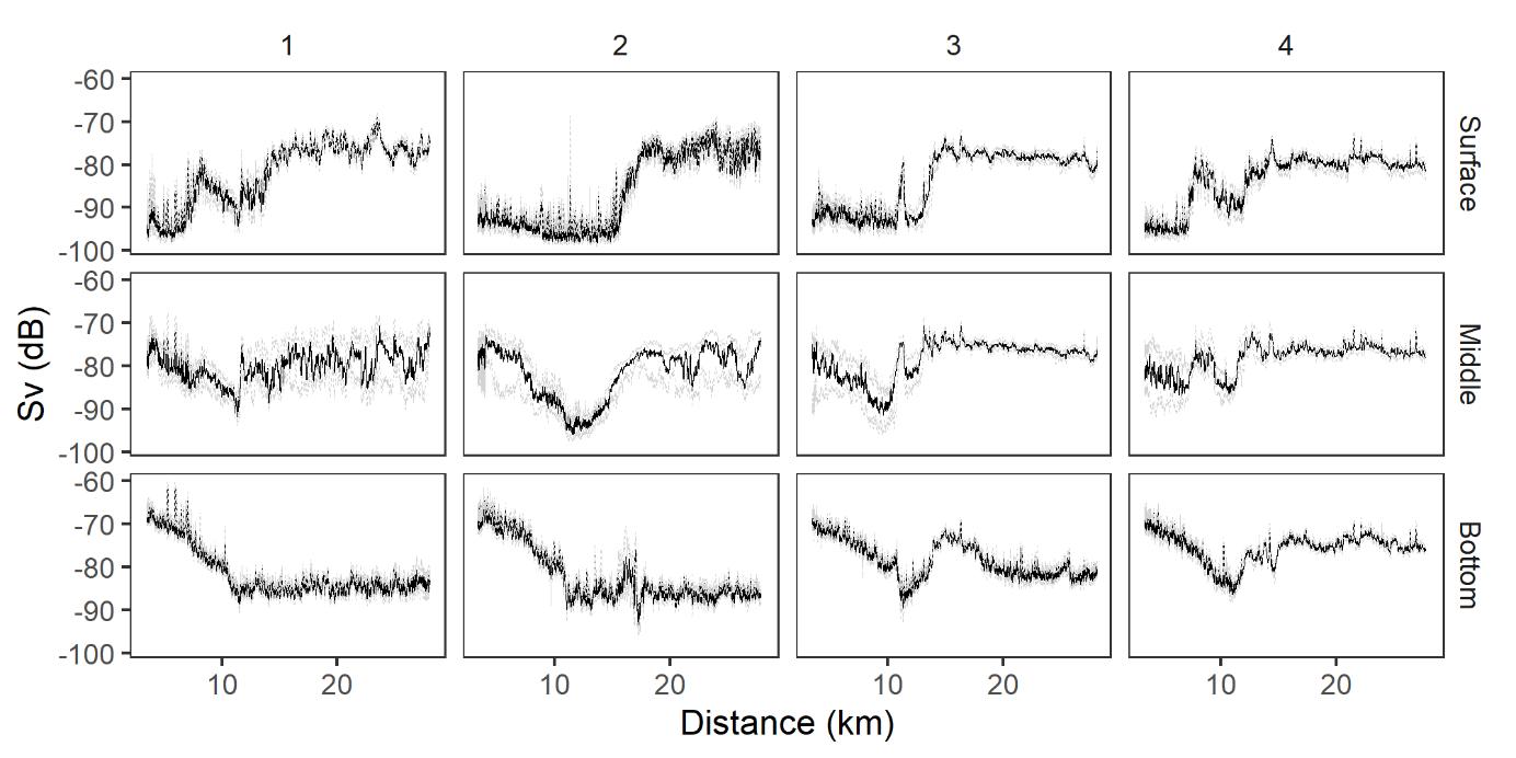
Figure 17. Acoustic backscatter registered in the southwestern (SW) transect. The data are presented as median Sv values (11 ping running median values) in the surface (top panels), middle (middle panels) and bottom (bottom panels) layers and with distance from the planned windfarm. Numbers 1:4 represent the four replicates Dashed light grey lines are the 25th and 75th quantiles.
5 - Discussion
The most abundant species caught during this survey, which are also of commercial interest, were ling, hake, saithe, cod and whiting. We found no significant changes in species diversity with distance to the windfarm site, but we found clear patterns in fish abundance of the most commonly caught species in this survey. Cod and ling were mainly caught in the shallower areas further away from the windfarm site, while hake and saithe were mainly caught in the deeper waters close to the windfarm site. Whiting was predominantly caught at a single station furthest from the windfarm site. Maturity, within these species did not vary with depth or distance to the windfarm site, except for ling, which showed a higher proportion of mature fish in the shallower areas. Cod, ling and saithe were larger in the deeper areas compared to the shallow areas. However, only 17 cod were found in the deeper areas. Hake were larger in the shallow areas compared to the deeper areas, but only 5 were caught in the shallow areas. Ling were in better condition in the shallow areas than in the deeper areas. Within these areas we found no consistent patterns in length and condition with distance to the wind farm site within these areas. The significant patterns found were based on few individuals per station and could be variable. However, these significant relations should be monitored in future cruises to assess how stable they are over time and whether they change with the age of the wind farm.
The fishing method used was aimed at catching bottom fish. However, stomach content analyses revealed some information about pelagic species, as well. In particular for mackerel, which was present in the stomachs at all stations. Only ling and saithe were found at all stations in sufficient numbers for stomach analyses. The stomach samples of these species should thus be a priority on future cruises after establishment of the windfarm. However, stomach samples from other species may be useful to include to see whether diet may change within the windfarm or in relation to movement towards the windfarm. Cod is a species that has been seen to spend time feeding in windfarms. Cod will therefore be a highly interesting species to monitor for abundance and diet after the establishment of the windfarm.
At current speeds of more than 0.8 knots, experience has shown that the type of net used on the cruise will be laid on the bottom and the catch efficiency will be reduced. We did not record such current speeds on this cruise. However, on two occasions, nets set in area 6 had moved up to 2.5 n miles due to current and probably poor attachment for the anchors on the bottom. Therefore, we moved station 6 to a new location and this new station should be used in follow up studies after establishment of the windfarm. All nets drifted a little, however, which led to an overlap in location between stations 1, 2 and 3 (Figure 3). Station 1 may also be too close to the nearest turbine to safely deploy the nets. Follow-up studies should carefully consider which of these stations to use.
In this survey the acoustic data collection was a second priority and needed to be adapted to the fishing trials and the instrumentation available on the vessel. All data were collected at nighttime when there was no fishing activity. Ideally it would have been useful to collect data also at daytime when fish behaviour may be different and their availability for acoustic detection may be different. The acoustic backscatter levels were generally low, and few registrations of individual targets or aggregations were made. However, acoustic backscatter close to surface (5 – 25 m below surface) was strongest in the shallower areas 10 – 20 nm southwest of the planned windfarm. Denser aggregations were also only registered in these shallower areas. Acoustic backscatter from near the seabed (5 – 25 m above seabed), on the other hand, was higher in the deeper areas, but this backscatter may have been caused by noise when using a relatively high frequency at longer range and may thus not result from marine organisms. With only one acoustic frequency, a system that was not calibrated and without ground truthing the acoustic data it will not be possible to allocate acoustic registrations to species. However, changes in the patterns in backscatter after establishment of the windfarm would reflect changes in marine organisms, it will thus be interesting to monitor the acoustic backscatter levels and trends during the construction and operational phases to see whether these change or remain the same. In follow up studies it will be important to follow the same survey design with the transect design, instrumentation and settings and time of day and year.
Gathering eDNA data was a third priority of the cruise. To compare the results of eDNA analyses and catches, it would have been ideal to collect eDNA samples from all stations and at least from the bottom water. However, the information from the obtained eDNA samples will give some background information about eDNA-detectable fish species before the construction started and if eDNA sampling is continued in follow-up studies during the construction and operational phases, changes in species richness may be detected – especially if eDNA sampling is expanded to include all stations in future cruises.
We gathered no quantitative data on seabirds during this cruise. However, we observed that seabirds gathered around the fishing vessels fishing in this area including ours. It is typical that large numbers of seabirds follow fishing vessels. It is thus conceivable that in a situation where fishing vessels fish close to wind turbines, the fishing vessels can take the birds to the turbines and that this can lead to seabirds being killed. This should additionally be monitored during future cruises.
6 - Acknowledgements
The survey was funded by Equinor and carried out by the Institute of Marine Research. Planning of the survey was done by the Institute of Marine Research in collaboration with Equinor, Fiskebåt and fishermen that are experiences in this area. Data analyses was conducted by IMR. We thank Kari Mette Mürvol and Jürgen Weissenberger (Equinor), Gjert Endre Dingsør (Fiskebåt, Norwegian Fishery Association) and August Fjeldskår (Nesefisk AS) for valuable comments on a previous version of this report.
7 - References
Equinor 2019. Hywind Tampen PL050 – PL057 – PL089 PUD del II – Konsekvensutredning
Methratta, E.T. 2021. Distance-Based Sampling Methods for Assessing the Ecological Effects of Offshore Wind Farms: Synthesis and Application to Fisheries Resource Studies. Front. Mar. Sci. 8:674594. doi: 10.3389/fmars.2021.674594
Miya M., Sato Y., Fukunaga T., Sado T., Poulsen J. Y., Sato K., Minamoto T., Yamamoto S., Yamanaka H., Araki H., Kondoh M. and Iwasaki W. 2015. MiFish, a set of universal PCR primers for metabarcoding environmental DNA from fishes: detection of more than 230 subtropical marine species. R. Soc. open sci. 2: 150088.
Mjanger, H., Svendsen, B.V., Fuglebakk, E., Skage, M.L., Diaz, J, Johansen, G.O., and Vollen, T., Bruck, S.A., Gundersen, S. 2022. Handbook for sampling fish, crustaceans and other invertebrates. Version 29. Ref.id.: FOU.SPD.HB-05, Institute of Marine Research. 146 pp.
Stoeckle, M.Y., Adolf, J., Charlop-Powers, Z., Dunton, K.J., Hinks, G., VanMorter, S.M., Trawl and eDNA assessment of marine fish diversity, seasonality, and relative abundance in coastal New Jersey, USA, ICES Journal of Marine Science, Volume 78, Issue 1, January-February 2021, Pages 293–304, https://doi.org/10.1093/icesjms/fsaa225
HAVFORSKNINGSINSTITUTTET
Postboks 1870 Nordnes
5817 Bergen
Tlf: 55 23 85 00
E-post: post@hi.no
www.hi.no