Brisling er en viktig del av økosystemet i mange norske fjorder, der fisk, fugl og sjøpattedyr beiter på den. For å kunne overvåke endringene i brislingbestandene og gi et bærekraftig kvoteråd på brisling, gjennomføres det regelmessige akustiske-tråltokt i fjordene med forskningsskip i regi av HI. Det har blitt stilt spørsmål ved kvaliteten på dataene som samles inn med disse skipene, da man har indikasjoner på at en del av brislingstimene står for nær overflaten til å kunne måles med skipets ekkolodd. I tillegg er det krevende å navigere nært land og på grunne områder med disse store skipene. Under brislingtoktet i 2021 med FF Kristine Bonnevie ble det derfor gjennomført et eksperiment der ekkoloddata (200 kHz) ble samlet inn med Havforskningsinstituttets stillegående kajakkdrone i sidearmer av Sognefjorden og Hardangerfjorden for å avdekke eventuelle forskjeller i fordeling og tetthet observert med henholdsvis skip og drone. Det ble videre gjort et forsøk for å studere eventuell fartøyunnvikelse ved at kajakkdronen drev over tette overflatekonsentrasjoner av brisling mens forskningsskipet passerte tett på med vanlig tokthastighet på 10 knop. På dagtid var de akustiske tetthetene like mellom plattformene. Kayak Drone (USV) registrerte imidlertid høyere akustiske tettheter om natten enn på dagtid. Denne forskjellen kan skyldes dybdeavhengige akustiske målstyrker, hvor målstyrken reduseres med dybden. FF Kristine Bonnevie registrerte lignende tettheter både dag og natt, men hadde en større akustisk blindsone fordi transduseren er plassert dypere (6 m mot 1 m for Kayak Drone). Dette påvirket den observerte vertikale fordelingen, slik at brisling ble observert dypere om natten med FF Kristine Bonnevie. En dykkereaksjon hos brisling når FFen passerte kan redusere målstyrken, noe som forklarer den lavere NASC-verdien. Fremtidige brislingundersøkelser med mindre USV-er må ta hensyn til plattformavhengige forskjeller i blindsone, fartøyunnvikelse og målstyrke.
Measuring distribution and density of sprat in Norwegian fjords using a kayak drone
Report series:
Rapport fra havforskningen 2025-11
ISSN: 1893-4536
Published: 18.02.2025
Updated: 21.02.2025
Project No.: 15977-02, 16181
Research group(s):
Pelagisk fisk
,
Akustikk og observasjonsmetodikk
Subject:
Brisling,
Droner og ny teknologi i havforskningen
Program:
Kystøkosystemer,
Norskehavet
Research group leader(s):
Espen Johnsen (Pelagisk fisk) og Rolf Korneliussen (Akustikk og observasjonsmetodikk)
Approved by:
Research Director(s):
Geir Huse
Program leader(s):
Bjørn Erik Axelsen, Halvor Knutsen og Even Moland
Norsk sammendrag
Summary
Sprat is a key species in several Norwegian fjords, as an important prey for fish, sea mammals and sea birds. The sprat populations are monitored with routine acoustic-trawl surveys using a large research vessel, which provides the main scientific basis for the sprat quota advice. Previous survey observations indicate that a significant fraction of the sprat population can be found close to the sea surface and thereby in the acoustic blind zone of the echo sounder mounted below the vessel. In addition, fish may avoid the approaching vessel, and thereby measure less acoustic density. Furthermore, a large research vessel cannot operate in shallow waters and is difficult to maneuver close to the shore. Experiments were carried out in several side arms of the Sognefjord and Hardangerfjord to identify any potential differences in observed distribution and density from the research vessel and the Kayak Drone. Furthermore, the kayak drone was drifting above dense concentrations of sprat close to the surface as the research vessel passed by at 10 knot survey speed. This was done to study potential vessel avoidance reactions. During the day, acoustic densities were similar across platforms. At night, however, the Kayak Drone (USV) recorded higher acoustic densities than during the day. This difference may be due to depth-dependent acoustic target strengths, where the target strength decreases with depth. The RV Kristine Bonnevie recorded similar densities both day and night but had a larger acoustic blind zone due to its deeper transducer (6 m versus 1 m for the Kayak Drone). This affected the observed vertical distribution, with sprat observed deeper at night with the RV Kristine Bonnevie. A diving response from sprat when the RV passed over could reduce target strength, explaining the lower NASC. Future sprat surveys with smaller USVs will need to account for platform-dependent differences in blind zones, avoidance, and target strengths.
1 - Introduction
Sprat is a key species in the Norwegian fjord ecosystems where it feeds on zooplankton (Falkenhaug and Dalpadado 2014) and is preyed upon by seabirds, fish, and sea mammals (Aarefjord et al. 1995, Solberg 2017, ICES 2024). To monitor the state of the sprat stocks in the fjords, the Institute of the Marine Institute carries out annual acoustic trawl surveys in the Sognefjord, Hardangerfjord and Nordfjord, and in some years in the Trondheimsfjord and Oslofjord. The survey areas are covered day and night based on the assumption of equal vulnerability to the echo sounders at any time of the day. The timing of the surveys has not been constant over the years, but since 2019 the surveys have been carried out in the summer and early autumn (July to September) using the research vessel Kristine Bonnevie (Stiti 2022). The main motivation for running the surveys in this period is to get an estimation of geographical distribution, individual length, abundance and biomass of the recruits (age 0) and older individuals (age 1+) close in time to the main fishing season in the autumn. The abundance and biomass estimates are not considered to reflect the absolute values of the stock, but the indices are assumed to reflect the trends in abundance and biomass which is used as input for the stock assessment and advisory process of sprat.
Technology advancement have led to a speedy development of uncrewed surface vehicles (USV) for marine ecosystem monitoring (Totland and Johnsen 2022), and the Institute of Marine Research aims to use small USVs in combination with research vessels to collect echo sounder data during the fjord sprat surveys by 2025. In this transition from using a research vessel to using USVs for data collection, it is important to examine how this change may affect the survey estimates.
Sprat undertakes diurnal migrations where they form schools in deep waters at daytime, and swim upwards at dusk and are distributed in layers near the surface at night. In the previous surveys, the acoustic data collection has been carried out using large research vessels with the echo sounder transducers mounted on a retractable keel, however, in the calm sea-state conditions in the fjords the keel has not been extended. Thus, the transducer depth has been approximately 6 m. The transducer depth on a USV is considerably shallower and can monitor fish closer to the surface than a large vessel. In addition, several studies show that clupeids tend to avoid an approaching large vessel by diving and/or swimming to the sides of the vessel. This behaviour results in a reduction of the measured acoustic density as less fish is observed within the beam of the echo sounder and as the downward swimming direction reduce the back scattering energy of individual fish within the beam. Totland and Johnsen (2022) show that herring does not avoid a small silent USV Kayak Drone, and a previous experiment in 2020 suggests that sprat has less avoidance to a silent USV Kayak Drone than a large research vessel (Johnsen et al. 2020). Also, a large research vessel, in contrast to a small USV, cannot operate in shallow waters. It is, furthermore, difficult to maneuver the ship very close to the shore. As shown by Johnsen et al. (2020), sprat may be distributed near the shore and in shallow waters, which may have caused biases in the survey time series.
To examine the potential platform-dependent differences in acoustic density recording of sprat described above, we carried out several experiments using the silent USV Kayak Drone and the RV Kristine Bonnevie in August and September 2021. The main objectives of this study were to answer the following questions:
Q1: Is the mean measured acoustic density of sprat in a fjord independent of the platform?
Q2: Is the mean measured acoustic density of sprat the same day and night, and is any day-night differences platform dependent?
Q3: Is the vertical distribution of acoustic density of sprat independent of the platform?
Q4: Does sprat show vessel avoidance to RV Kristine Bonnevie?
2 - Materials and methods
2.1 - Platform comparison experiments
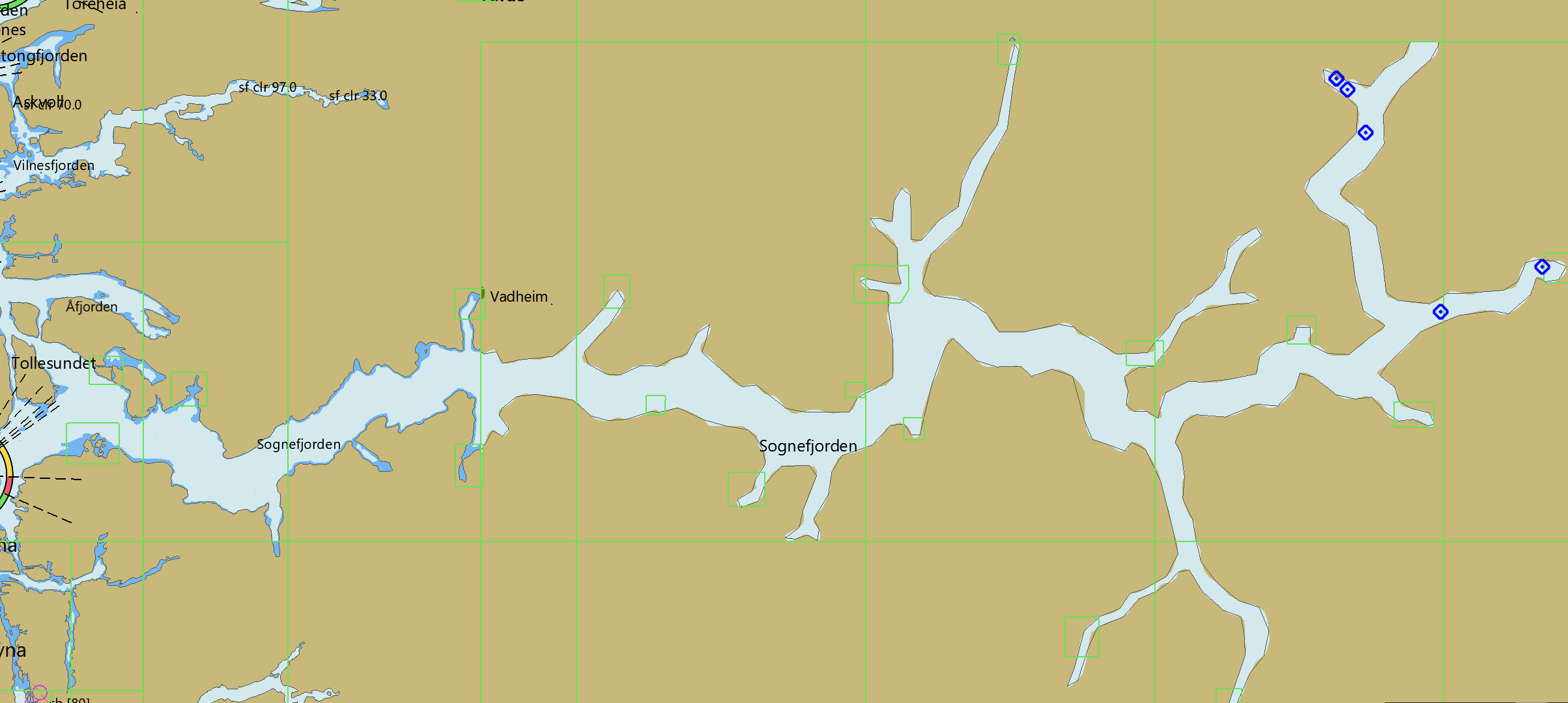
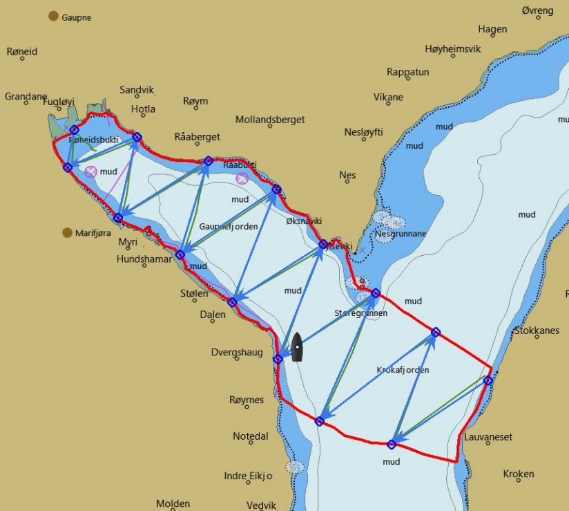
To examine questions 1-3 above, we defined three strata in the fjords. The first stratum was the same as covered during the 2020 survey (Johnsen et al. 2020). However, the density of sprat in this stratum (Årdalsfjord; a side arm of Sognefjord) was very low, and it was therefore decided to cancel the night coverage to save survey time. The other two strata were based on preliminary examination of the density of sprat carried out by RV Kristine Bonnevie (survey numbers 2021619 and 2021621). Each stratum was covered both night and day with zigzag transects. In each coverage, the Kayak Drone was followed by RV Kristine Bonnevie at a minimum distance of 500 m.
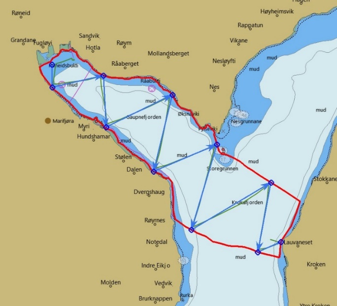
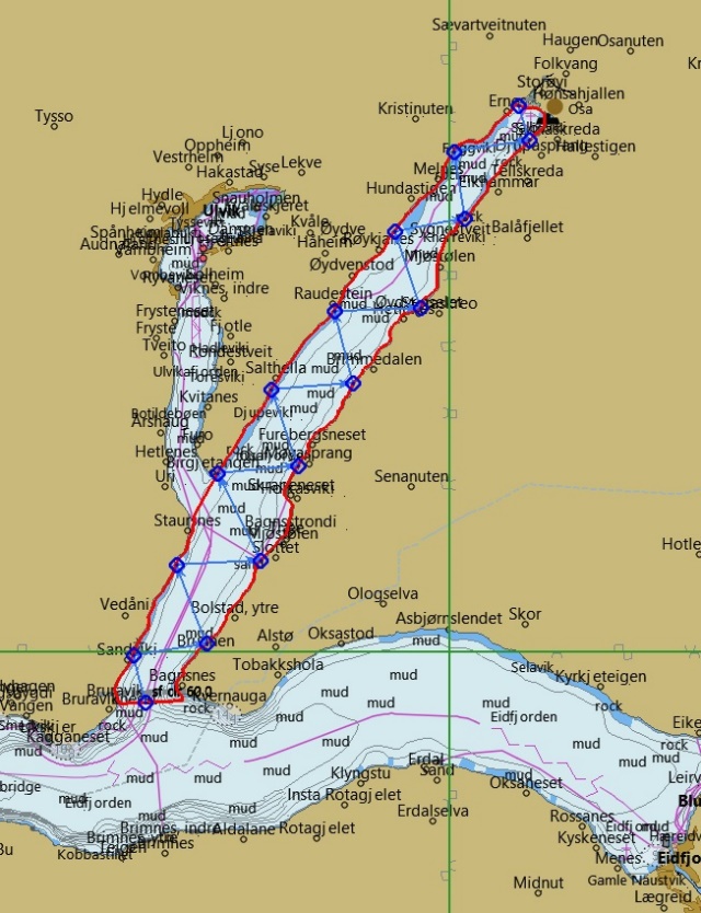
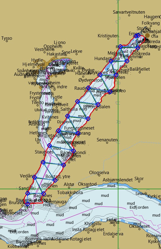
Each stratum polygon was defined using the same method as in 2020 (Johnsen et al. 2020). We downloaded high resolution map data from Kartverket (https://www.kartverket.no/), and the following procedure was used to generate a stratum and survey transects: The high-resolution map was loaded into the map program OpenCPN (https://opencpn.org/). In OpenCPN, a closed route (GPX format) was made interactively for each fjord, with the outer boundaries 30 m from the shore. An R script was made to convert the GPX route to a WKT polygon stratum file which is used by the surveyPlanner function in the R-package Rstox 1.11.1 (https://www.hi.no/hi/forskning/prosjekter/stox/). For each run, the Rstox::surveyPlanner was used to generate evenly distributed transects with a random start position in a zig-zag pattern across the fjord. Figures of the strata borders and transects for each run are presented in Appendix 6.1 (Figures A1.1-A1.5), and Table 1 show the time and sailing distances of each stratum coverage.
| Survey | Main fjord | Fjord arm | Area (nmi2 ) | Time (UTC) | Sailing distance (nmi) |
| 1 | Sognefjord | Årdalsfjord | 9.86 | Day: 31/8-21 14:15 – 17:44 | 15.2 |
| 2 | Sognefjord | Gaupnefjord | 2.97 | Day: 01/9-21 07:50 – 10:40 | 11.3 |
| 3 | Sognefjord | Gaupnefjord | 2.97 | Night: 01/9-21 19:05 – 21:05 | 7.9 |
| 4 | Hardangerfjord | Osafjord | 3.83 | Night: 05/9-21 20:00 – 22:42 | 10.6 |
| 5 | Hardangerfjord | Osafjord | 3.83 | Day: 06/9-21 08:25 – 11:40 | 14.7 |
2.2 - Acoustic data recording, scrutinizing and acoustic categorization
Data was recorded with Simrad EK80 echo sounders on both Kristine Bonnevie and the Kayak Drone. The echo sounder settings were as described in chapter “Echo sounder calibration and EK80 settings”. For the Kayak Drone, a draft of 1 m was applied in the EK80 software, while Kristine Bonnevie had a draft of 6 m, both referring to the depth of the transducer. Both vessels conducted the surveys at a speed of approximately 5 knots. Acoustic data was collected down to 150 m using a ping interval of 370 and 520 ms for the Kayak Drone and Kristine Bonnevie, respectively. 150 m depth was assumed to be below the maximum vertical distribution of sprat, based on previous survey recordings.
Raw acoustic data (200 kHz) was scrutinized in LSSS 2.15 software (Korneliussen et al. 2016). Prior to assigning values to the only acoustic category, SPRAT, all backscatter noise and bottom echoes were excluded. Data was stored at a 1-m depth resolution at an integrator distance of 0.1 nmi. A threshold of -55 dB was applied to remove echoes from plankton. The scrutinized sprat data was exported in units of Nautical Area Scattering Coefficient (NASC; m2 nmi-2) to an NMDechosounder.xml file which is stored in the NMDechosounder database at IMR.
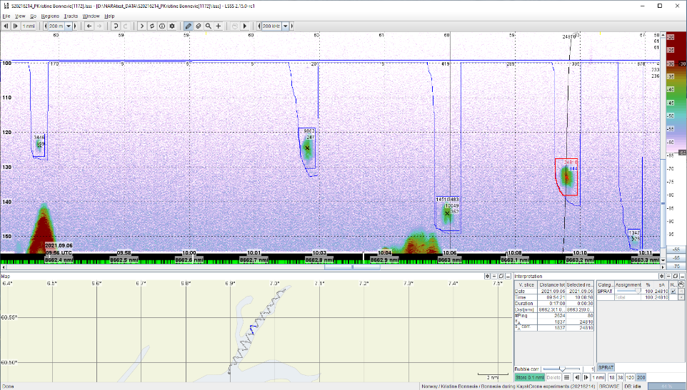
From the draft depth of each vessel and down to 100 m, a layer was used for the interpretation. Below 100 m, the background noise increased on both vessels and only school boxes were used (Figure 1). In this deeper waters, scatter layers of sprat did not occur, only schools and only during daytime in Osafjord and Årdalsfjord. The sprat NASC data extracted from the recordings in LSSS was used for the analysis.
2.3 - Data analysis of acoustic density
For each of the surveys (Table 1), a StoX project (Johnsen et al. 2019) was created for both the Kayak Drone run and the Kristine Bonnevie run. The respective NMDechosounder.xml from LSSS was imported into the StoX project. In StoX, the transects were defined as acoustic primary sampling units (PSU). All further analyses were carried out in R (R Core Team 2024). For each of the surveys, we calculated the weighted mean NASC by platform.
To estimate the mean and variance of the NASC values, we use the methods established by Jolly and Hampton (1990). The primary sampling unit is the weighted mean of all elementary NASC samples of sprat along the transect, where the distances of the elementary samples are used as the weighting variable. The transect (t) has NASC value (s) and distance length L . The average NASC (S) in a stratum is:
 (1)
(1)
where  (t= 1,2,..,ni ) are the weights based on the lengths of the n sample transects, and
 (2)
(2)
Variance by stratum is estimated as:
 with
with  (3)
(3)
We compared the mean stratum density by platform, and day-night differences in mean acoustic density within and between platforms.
To compare the vertical distribution of the acoustic density of sprat by stratum, platform and between day and night, we estimated the weighted depth distribution (Avgnasc) by survey and platform as:
 (4)
(4)
where NASC and Depth are the NASC and Depth values by 1-m and 0.1 nmi sailing distance by survey and platform.
2.4 - Research vessel avoidance experiment
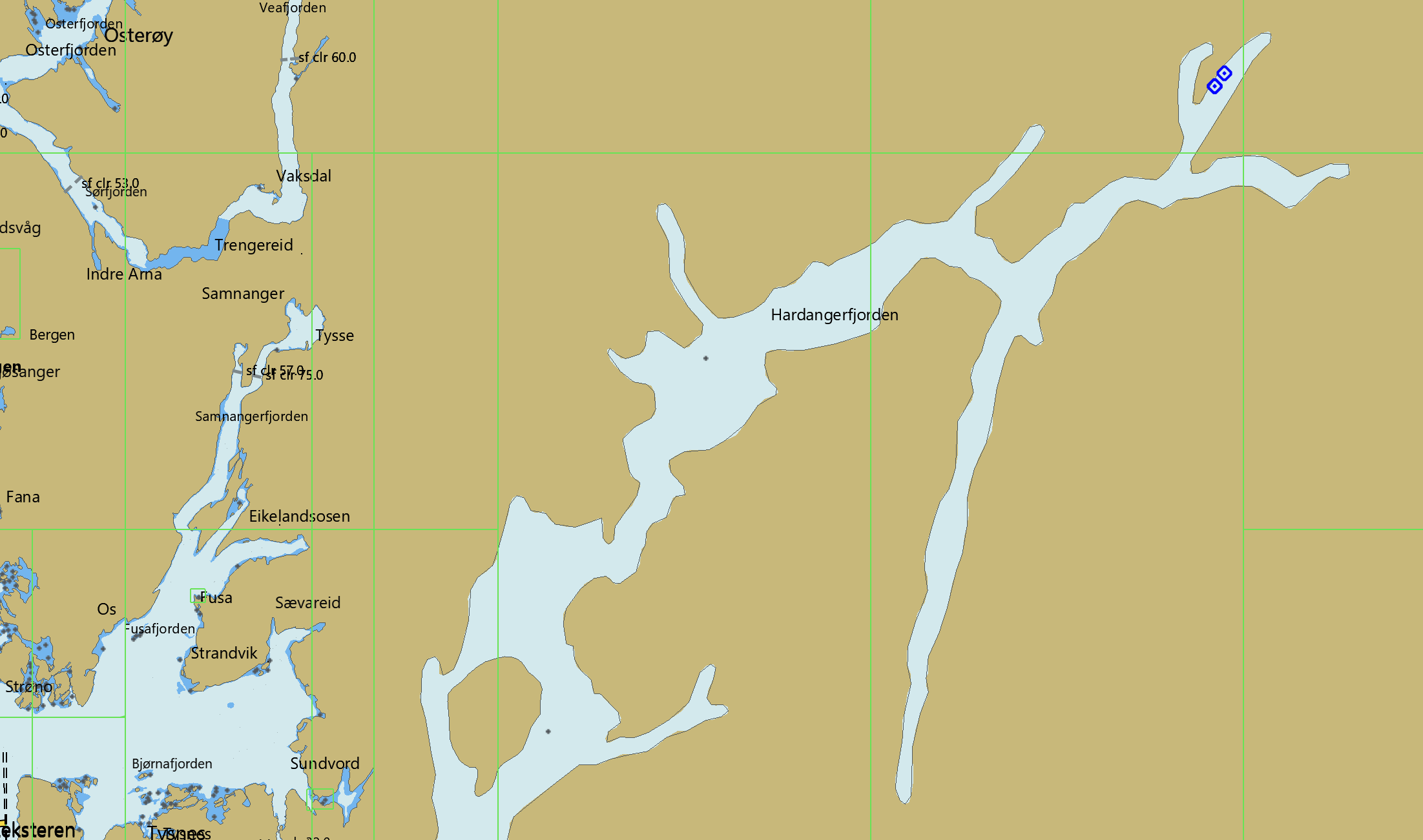
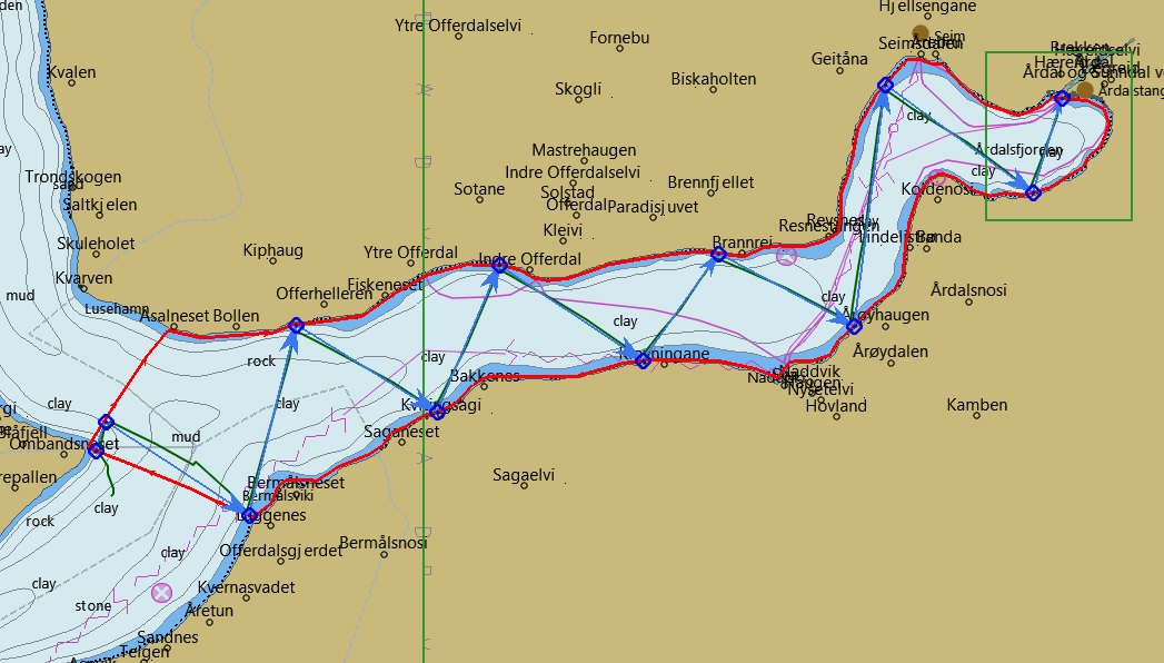
To examine potential research vessel avoidance of sprat close to the surface, we carried out an experiment in Osafjord, close to the mouth of Ulvikafjord in the Hardangerfjord, on September 6 after sunset (Figure 2). A successful experiment was dependent on identifying locations with high densities of sprat, and the Kayak Drone was used to search for dense concentrations of sprat near the sea surface. Upon detecting high sprat densities, the Kayak Drone was laid to rest and drifted in the high-density area. Thereafter, we established a sailing route transect with RV Kristine Bonnevie to pass the drifting Kayak Drone at standard survey speed as close as possible to the port-side of the research vessel (Table 2). This experiment was repeated seven times, and the location of the Kayak Drone was changed between each passing (Figure 2). The EK80 data were recorded continuously on the Kayak Drone, and the EK80 200 kHz on the research vessel was set to passive to avoid interference.
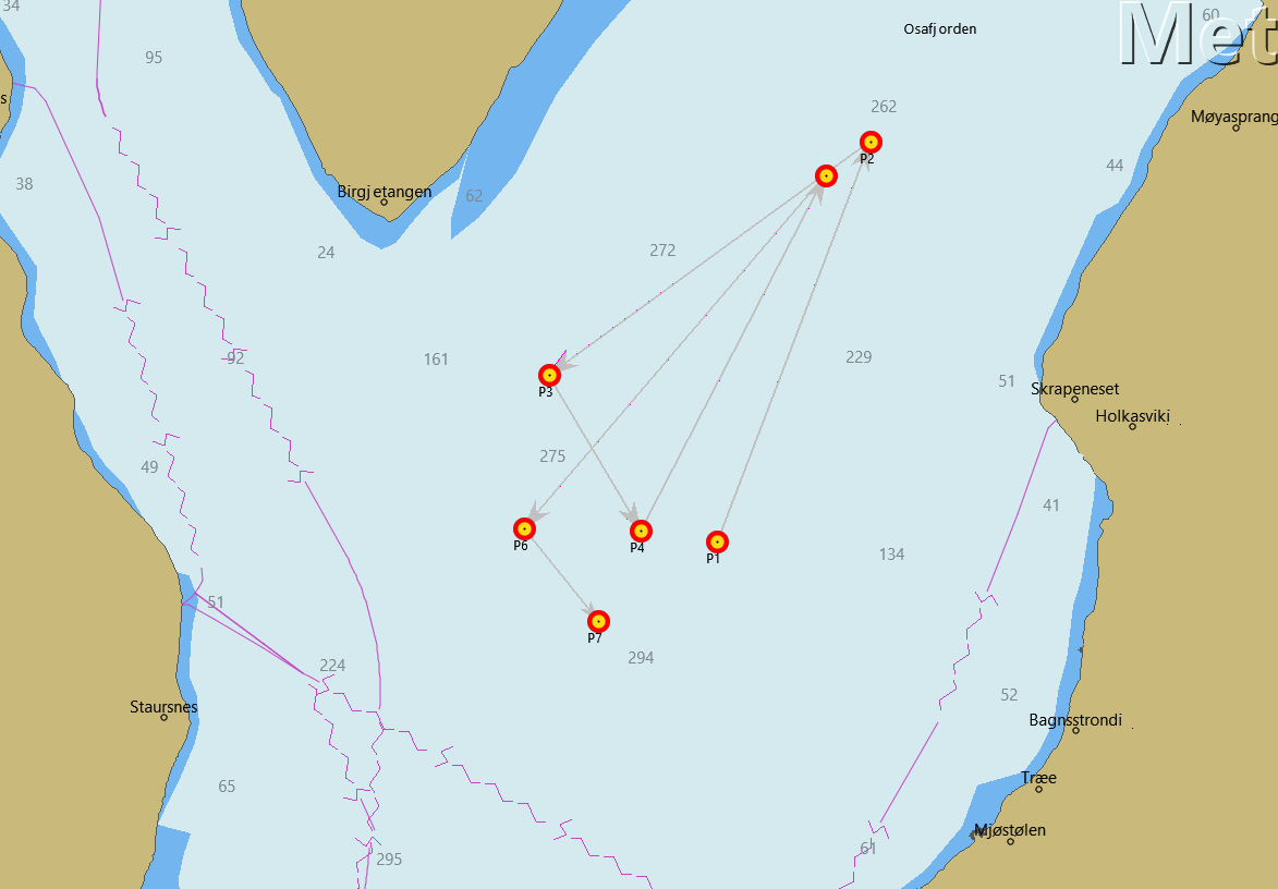
| Pas # | Time | Latitude | Longitude | Distance (m) | Speed (knots) |
| P1 | 20:02:30 | 60°31.2759 ˈ N | 6°56.1655 ˈ E | 18.0 | 6.7 |
| P2 | 20:30:18 | 60°31.7307 ˈ N | 6°56.4437 ˈ E | 15.9 | 7.7 |
| P3 | 20:47:58 | 60°31.4807 ˈ N | 6°55.7527 ˈ E | 23.1 | 8.5 |
| P4 | 21:06:59 | 60°31.2966 ˈ N | 6°55.9983 ˈ E | 27.3 | 8.1 |
| P5 | 21:23:50 | 60°31.7084 ˈ N | 6°56.3691 ˈ E | 36.6 | 8.3 |
| P6 | 21:43:56 | 60°31.2846 ˈ N | 6°55.7221 ˈ E | 13.2 | 8.2 |
| P7 | 21:56:03 | 60°31.2265 ˈ N | 6°55.9160 ˈ E | 18.7 | 7.8 |
2.5 - Echo sounder calibration and EK80 settings
2.5.1 - EK80 settings
Kristine Bonnevie and the Kayak Drone are both equipped with an EK80 transceiver and an ES200-7C transducer. The following transceiver settings were used during the survey and the calibration for both Kristine Bonnevie and the Kayak Drone:
FrequencyStart = 162 kHz
FrequencyEnd = 258 kHz
PulseLength = 2.048 ms
PulseForm = LFM
Slope = 0.6028 %
TransmitPower = 105.00 W
SampleInterval = 0.008 ms
2.5.2 - Calibration
The EK80 echo sounders were calibrated prior to surveying (Figure 3). It was only calibrated in FM mode (broadband) as this was the mode to be used by both the Kayak Drone and RV Kristine Bonnevie. A 35 mm tungsten sphere was used for the calibration and the transceiver settings were in accordance with advice from acoustic experts (same settings in the Kayak Drone and RV Kristine Bonnevie).
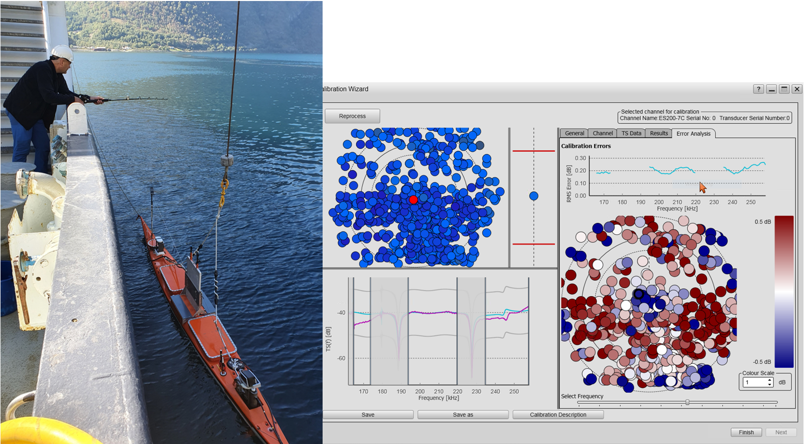
The Kayak Drone was lifted onto the sea by the deck crane and kept 2 m out from the ship side. The calibration sphere was lowered to approx. 18 m depth, using a standard fishing rod. The sphere was moved throughout the beam by tilting the drone sideways by dragging and pushing the crane wire, and by moving the fishing rod along the side of the USV.
RV Kristine Bonnevie was calibrated prior to the annual coastal sprat survey using standard procedures for research vessels. The Kayak Drone experiment was a part of the coastal sprat survey.
2.6 - Description of the Kayak Drone
The Kayak Drone has undergone some upgrading after the 2020 coastal sprat survey (Johnsen et al. 2020):
-
The most significant upgrade is the replacement of the radio link with a Kongsberg Maritime Broadband Radio (MBR). MBR is an advanced system frequently used in military applications. With the new radio link in place, the remote operation is reliable and problem free over both short and long range. For this reason, the remote operation could be set up in the wheelhouse of RV Kristine Bonnevie instead of onboard the small work boat as in 2020.
-
In 2020 we experienced some leakage. All leakage points have been found and repaired. No incident of leakage occurred this year.
2.6.1 - Technical issues
During the survey no consequential problems occurred, and all the surveys and experiments were conducted according to the plan. Some minor issues were discovered, and these were all identified and corrected shortly after the survey:
-
At one waypoint, the USV steered in a slightly wrong direction. It was discovered that this can happen in rare occasions due to a programming error in two subroutines of the EchoDrone program. The bug was identified after replaying the EchoDrone data from the survey. A new corrected software version is made.
-
The OpenCPN once shifted to the next waypoint approx. 90 m to early. This also occurred in one run in 2020. This is identified as a bug in the OpenCPN software. A description of why this sometimes happens and how to overcome the problem is now included in the Kayak Drone manual.
-
For night operations, we observed that a proper set of lanterns should be installed. This was corrected after the survey (green, red, and blinking white lights are now installed).
-
The crane lifting rope sometimes drop into the sea after deployment and is thus dragged through the sea. A rubber band rope was mounted to the lifting rope after the survey to avoid this.
-
EK80 SW blocks all serial ports on the USV if the program is started before the EchoDrone program. The settings in EK80 SW have been altered to avoid this.
-
The Torqeedo engine stops at an RPM (revolutions per minute) somewhere between 470 and 500. The engine must be set to 0 RPM before restart. This is a known bug in the Torqeedo firmware that easily can be corrected in the EchoDrone software when the exact failing RPM is identified. This identification must be done at sea since running the motor at such a high RPM in air may cause damage.
2.7 - Biological data
In each of the three strata (Gaupne, Årdal, Osa), at least two pelagic trawl hauls were carried out (Figure 4; Table 4). A Harstad trawl mounted with a codend with a small-meshed inner layer (mesh size: 8 mm) was used. The headrope of the trawl was equipped with depth sensors and a trawl eye. The width and height of the trawl opening were 20 m and 15 m, respectively. Target trawling was decided based on the acoustic backscattering densities, and trawling speed was about 3 knots.
The trawl catches were sorted and sampled using standard IMR procedures (Mjanger et al. 2025). When the catch was manageable, it was weighed by filling baskets and weighing all of them. Very large catches were weighed on deck by weighing the codend (both with and without catch). The catches were sorted by first taking out jellyfish and larger-sized fish (like e.g. saithe, pollock, dogfish, lumpfish, mackerel and large herring etc.) from the entire catch. Smaller-sized fish (sprat, small herring, stickleback, 0-group fish etc.) and zooplankton were subsampled unless catches were small. When catches were large, the subsample was taken from the beginning, middle and end of the catch.
Sprat and herring were targeted species for this survey, and for these full individual sampling of 30 individuals was done: total length (nearest 0.5 cm), round weight (g), sex, stomach fullness, age (from reading otoliths), and for herring also maturity, mesenteric fat and Ichthyophonus, whereof the last two parameters are not standard for IMR sampling of sprat. The maturity of sprat was not examined as it is not possible to reliably assess this in late summer. Further, up to 70 more individuals were measured and weighed. Other fish species were length measured. When two size groups were present (i.e. 0-group and possibly older sprat (herring)), sprat (herring) was sorted into two groups and sampled by group. Sprat smaller than 7 cm are all assumed to be 0-year-olds, and thus otoliths are only taken from 10 individuals for verifying this.
When sprat individuals weigh less than 1 g, it is not possible to get individual weight due to the resolution of the scales in the laboratory. The average weight can be calculated by dividing the sample weight by the number of sampled individuals. In future surveys, it could be an alternative to group the sample into length classes by 0.5 cm and weigh and count each length class group.
3 - Results
3.1 - Platform comparisons
The acoustic density (NASC) of sprat in Årdalsfjord, a side arm of Sognefjord, was very low and therefore the planned night coverage was cancelled. Full day versus night and research vessel versus Kayak Drone comparisons were carried out in Gaupnefjord (Sognefjord) and Osafjord (Hardangerfjord). At daytime, the mean acoustic density of sprat was not significantly different between the two platforms in these two fjords (Table 3). Furthermore, the density of sprat was not significant different between day and night coverages carried out by RV Kristine Bonnevie. In contrast, for the Kayak Drone the mean density measured at night was 2.0 and 6.3 times higher than the daytime measurements, respectively, in the Gaupnefjord and Osafjord surveys (Table 3).
| Platform | Day/night | Area | Mean NASC | NASC 5% | NASC 95% | RSE | Median depth |
| Kayak | Day | Gaupnefjord | 339 | 234 | 444 | 0.19 | 8 |
| KB | Day | Gaupnefjord | 380 | 53 | 708 | 0.52 | 14 |
| Kayak | Night | Gaupnefjord | 677 | 416 | 939 | 0.23 | 4 |
| KB | Night | Gaupnefjord | 280 | 163 | 398 | 0.25 | 11 |
| Kayak | Day | Osafjord | 330 | 91 | 570 | 0.44 | 103 |
| KB | Day | Osafjord | 460 | 121 | 799 | 0.45 | 131 |
| Kayak | Night | Osafjord | 2071 | 1283 | 2860 | 0.23 | 9 |
| KB | Night | Osafjord | 596 | 390 | 802 | 0.21 | 12 |
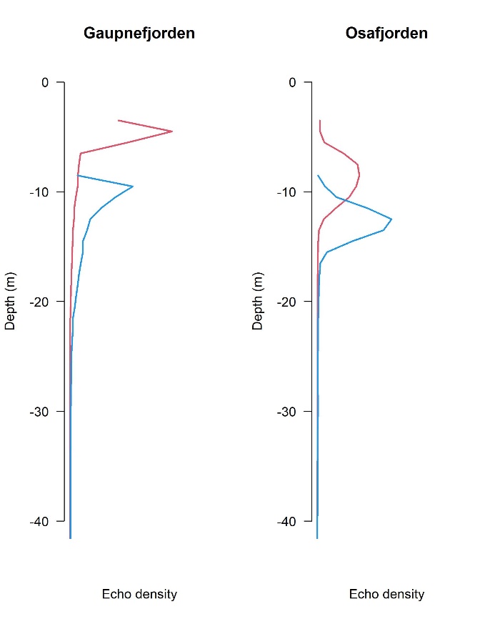
Sprat was distributed deeper at daytime than at night in both fjords (Table 3), however, the vertical density distribution of NASC at night differs markedly between the two platforms (Figure 5). The Kayak Drone observed sprat considerably closer to the surface than RV Kristine Bonnevie, where the peak sprat density observed with the Kayak Drone were at 4 m and 9 m depth, respectively, in the Gaupnefjord and Osafjord at night. The peak sprat density observed with RV Kristine Bonnevie were at 11 m and 12 m depths, respectively, in the Gaupnefjord and Osafjord.
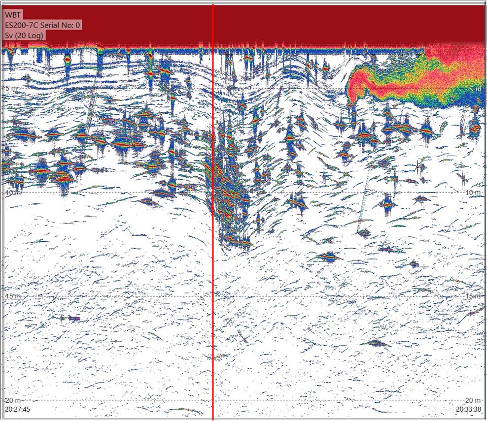
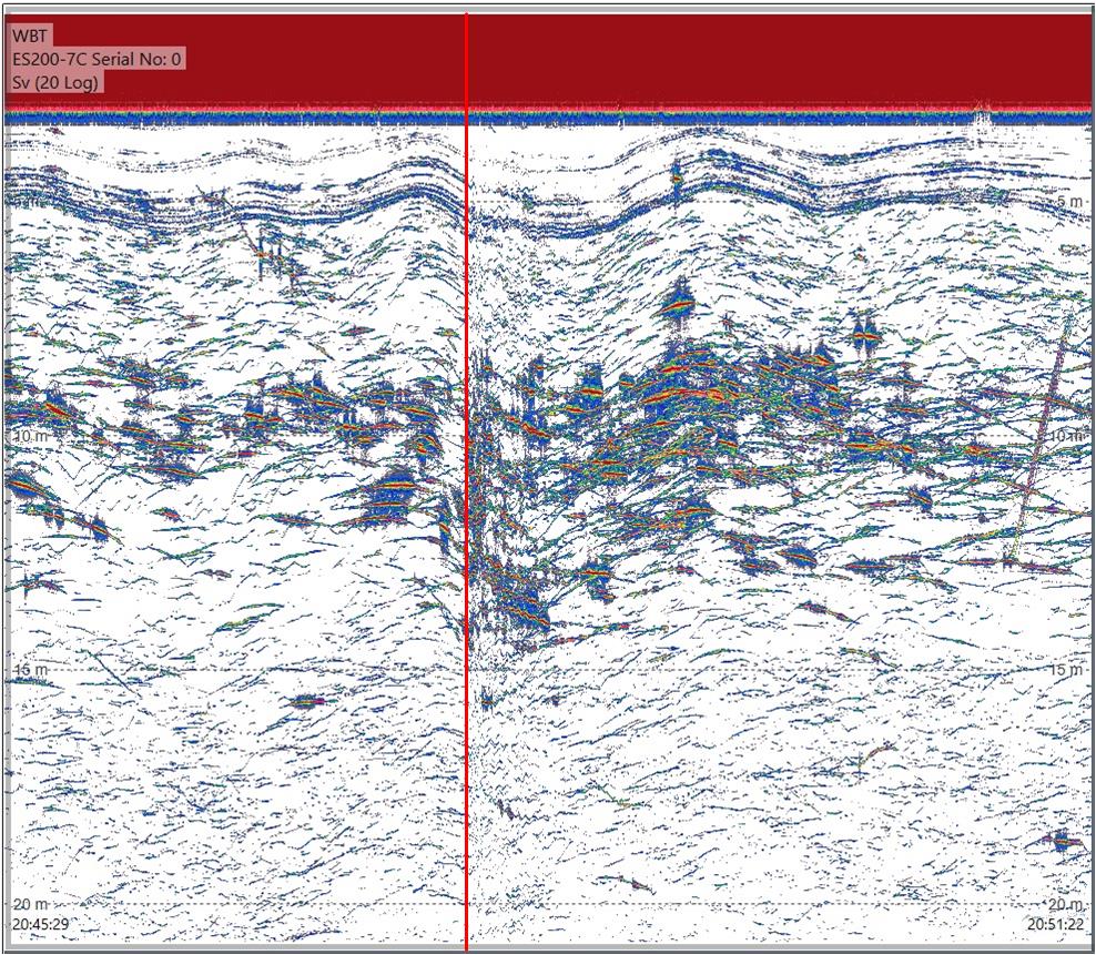
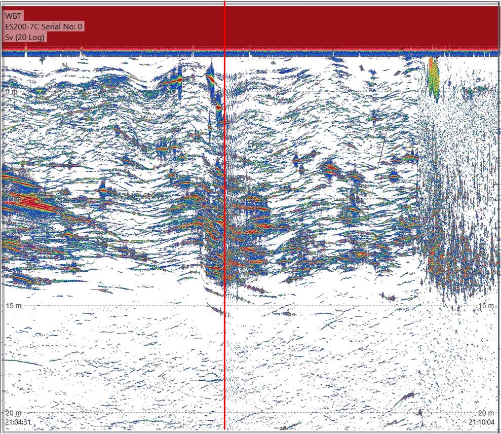
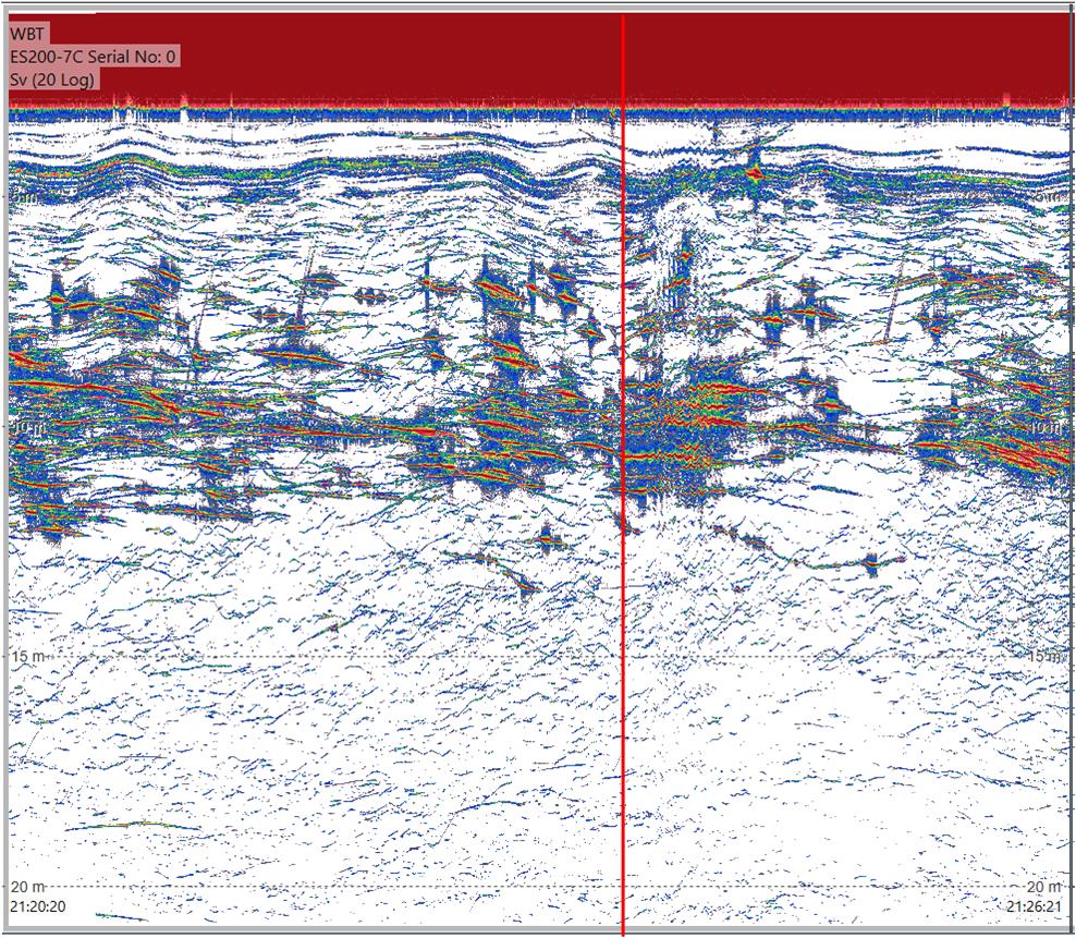
3.2 - Vessel avoidance
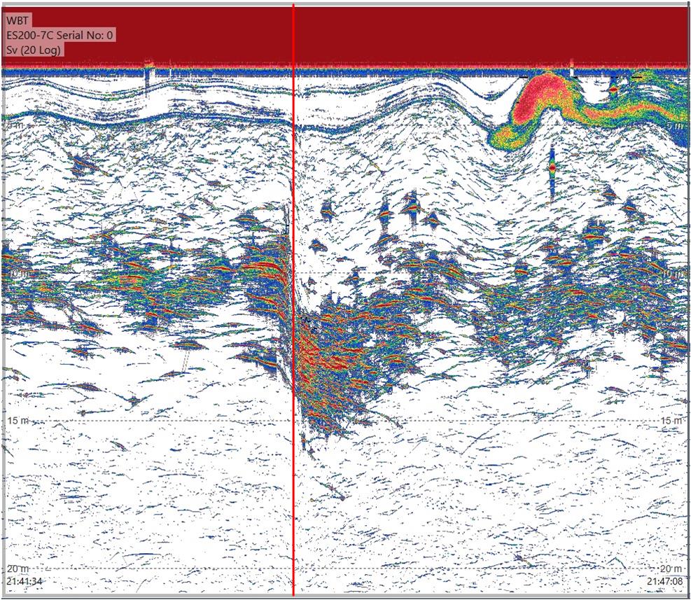
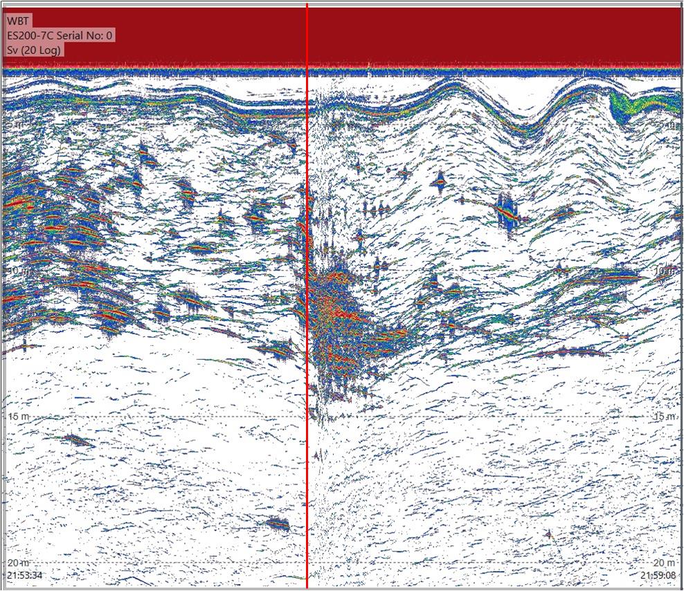
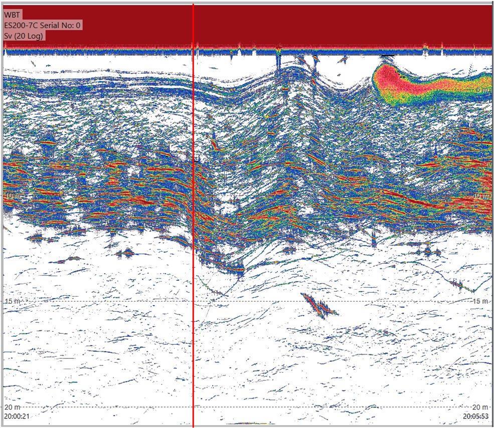
The research vessel passed the Kayak Drone at a standard survey speed of ~8 knots, and the minimum distance between the GPS of the Kayak Drone and the research vessel were in the range of 13 to 37 m during the passings (Table 2; Appendix 6.2: Figures A2.1-A2.6). The passing distance is very close and by visual inspection, the distance between the Kayak Drone and port side of the research vessel is estimated to be between 5-20 m. In all passings, the echograms showed that the sprat reacted to the research vessel when the distance was very short, however, no reaction was observed before the research vessel passed the Kayak Drone. When passing, the sprat individuals seemed to dive between 1-6 m (Figure 6; Figures A2.1-2.6).
3.3 - Trawl catches
Sprat were the fish dominating in the trawl catches (Gaupne: 55%, Årdal: 25%, Osa: 91% of the total catch weights) and were present in six out of seven trawl hauls (Table 4). Herring (G: 21%, Å&O < 1%) and spiny dogfish (G: 8%, O: 2%, Å < 1%) contributed less to total catches, but were present in five hauls each. One of the trawl hauls missed the target, and the catch was mainly jellyfish.
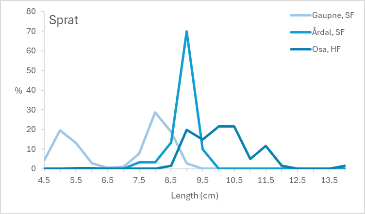
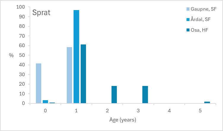
In Gaupne, both 0- and 1-year-old sprat were found (Figures 7-8). Both age groups had a lower length-at-age compared to Årdal and Osa. 1-year-old sprat dominated in Årdal (97%) and Osa (61%). In Osa, also older sprat (2-, 3- and 5-year-olds) were found (38%).
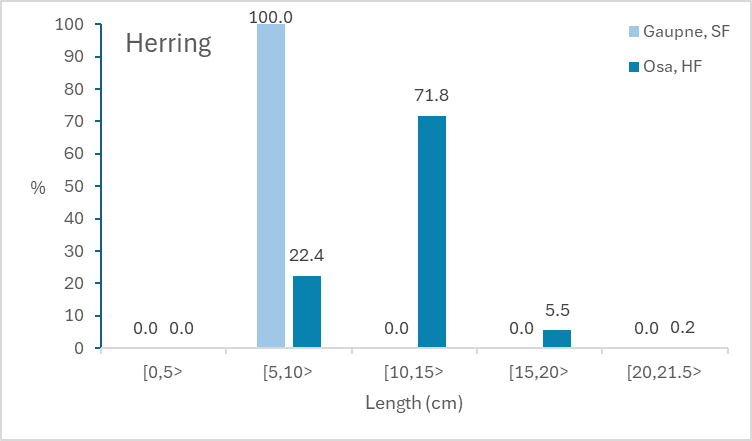
Herring were found in all three areas, but only one individual in Årdal (Figure 9). In Gaupne, only 0-winter-ringer (wr) herring (5-10 cm) was found, whereas in Osa 10-15 cm herring (also 0 wr) dominated (72%).
In the dark, zooplankton, like krill and Myctophidae, were found in the catches from the surface trawl hauls (Table 4).
| Strata (Fjord arm) | Gaupne (SF) | Årdal (SF) | Årdal (SF) | Gaupne (SF) | Gaupne (SF) | Osa (HF) | Osa (HF) |
| Serial number | 22566 | 22568 | 22570 | 22571 | 22572 | 22583 | 22585 |
| Date | 29 Aug | 30 Aug | 31 Aug | 1 Sep | 1 Sep | 5 Sep | 5 Sep |
| Time (UTC, hh:mm) | 21:18 | 21:46 | 18:15 | 11:35 | 15:32 | 02:32 | 23:16 |
| Max fishing depth (m) | 11 | 13 | 12 | 36 | 184 | 10 | 29 |
| Latitude start (°) | 61.386 | 61.193 | 61.230 | 61.377 | 61.342 | 60.545 | 60.553 |
| Longitude start (°) | 7.314 | 7.494 | 7.669 | 7.333 | 7.365 | 6.961 | 6.974 |
| Latitude stop (°) | 61.378 | 61.200 | 61.211 | 61.358 | 61.319 | 60.530 | 60.549 |
| Longitude stop (°) | 7.333 | 7.552 | 7.626 | 7.377 | 7.331 | 6.942 | 6.967 |
| Trawl distance (nmi) | 0.8 | 1.7 | 1.9 | 1.8 | 1.7 | 1.0 | 0.3 |
| Catch weight (kg) | |||||||
| Sprat | 19.126 | 41.944 | 170.739 | 19.723 | 1743.267 | 137.028 | |
| Krill | 14.294 | 43.170 | 2.838 | 19.420 | 29.880 | ||
| Lion's mane jellyfish | 5.540 | 21.152 | 48.100 | 6.122 | 4.870 | 7.420 | 13.526 |
| Herring | 66.819 | 0.015 | 11.772 | 4.457 | 0.387 | ||
| Spiny dogfish | 30.054 | 0.119 | 2.161 | 32.852 | 17.730 | ||
| Helmet jellyfish | 40.040 | 8.880 | |||||
| Myctophidae | 19.427 | 3.904 | 3.150 | 0.069 | |||
| Whiting | 4.850 | 4.019 | 2.358 | 0.042 | 0.021 | 1.871 | 1.868 |
| Lumpfish | 0.304 | 0.586 | |||||
| Mueller's pearlside | 0.549 | 0.089 | |||||
| Octopus | 0.600 | 0.017 | |||||
| Haddock | 0.013 | 0.392 | 0.023 | 0.012 | 0.008 | 0.044 | |
| Mackerel | 0.271 | 0.057 | |||||
| Blue whiting | 0.039 | 0.017 | 0.021 | 0.080 | |||
| Stickleback | 0.116 | ||||||
| Moon jelly | 0.046 | ||||||
| Syngnathiformes | 0.003 | ||||||
| Total catch | 160 | 115 | 51 | 191 | 31 | 1850 | 210 |
4 - Discussion and future plans
This study aimed to examine how the acoustic density of sprat in Norwegian fjords is affected by the observation platform, and these experiments are a follow-up of the study carried out in 2020 (Johnsen et al. 2020). During daytime the acoustic densities seem to be independent of the platform, however, the Kayak Drone measured considerably higher acoustic densities at night than at daytime. The higher NASC may be explained by depth dependent target acoustic target strengths, where the acoustic target strength decreases with depth (Ona 2003)
In contrast, the RV Kristine Bonnevie measured about the same acoustic density of sprat day and night. The acoustic surface blind zone is much larger for the RV Kristine Bonnevie than for the Kayak Drone as the transducer depths are ~6 m and 1 m, respectively. The difference in blind zone is also supported by the observed platform dependent differences in the vertical distribution of acoustic densities of sprat. At night sprat was observed at 3 m depth and deeper with the Kayak Drone, whereas the RV Kristine Bonnevie observed sprat from 8 m and deeper. Furthermore, the vertical distribution in NASC was markedly shallower for the Kayak Drone observations (Figure 6). The larger blind zone can explain the significant difference in NASC between the two platforms, however, our avoidance experiments show that sprat in the surface layer tend to dive several meters when the RV Kristine Bonnevie is passing over. Such a diving response is very common for clupeids (De Robertis and Handegard 2013), and often herring dive considerably deeper than what we observed for sprat in our experiment. A diving reaction may herd sprat down to a depth below the transducer depth, nevertheless, a diving reaction will also largely weaken the individual target strength due to a shift in the individual tilt and reduced swim bladder volume (Pedersen et al. 2024). Therefore, it is possible that the lower NASC values observed from RV Kristine Bonnevie compared to the Kayak Drone at night is a combination of the extent of the surface blind zone and reduced acoustic target strengths.
The Institute of Marine Research plans to carry out future sprat surveys using smaller USVs, and to be able to compare historical survey estimates with these future survey estimates there is a need to understand and compensate for platform dependent differences in surface blind zone, avoidance and target strengths.
5 - References
Aarefjord, H., Bjørge, A., Kinze, C.C. and Lindstedt, I. 1995. Diet of the harbour porpoise ( Phocoena phocoena ) in Scandinavian waters. Rep. int. Whal. Comm (Special issue16): 211-222.
De Robertis, A., and Handegard, N. O. 2013. Fish avoidance of research vessels and the efficacy of noise-reduced vessels: a review. ICES Journal of Marine Science 70: 34–45.
Falkenhaug, T., and Dalpadado, P. 2014. Diet composition and food selectivity of sprat (Sprattus sprattus) in Hardangerfjord, Norway. Marine Biology Research 10: 203-215.
ICES. 2024. Working Group on Multispecies Assessment Methods (WGSAM; outputs from 2023 meeting). ICES Scientific Reports. 6:13. 218 pp. https://doi.org/10.17895/ices.pub.25020968
Johnsen E., Totland A., Kvamme C. 2020. Measuring distribution and density of sprat in Årdalsfjorden with a Kayak Drone. Rapport fra Havforskningen Nr. 2020-28. https://www.hi.no/en/hi/nettrapporter/rapport-fra-havforskningen-en-2020-28
Johnsen, E., Totland, A., Skålevik, Å., Holmin, A. J., Dingsør, G. E., Fuglebakk, E., and Handegard, N. O. 2019. StoX: An open source software for marine survey analyses. Methods in Ecology and Evolution 10: 1523–1528.
Jolly, G. M., and Hampton, I. 1990. A stratified random transect design for acoustic surveys of fish stocks. Canadian Journal of Fisheries and Aquatic Sciences 47(7): 1282-1291.
Korneliussen, R. J., Heggelund, Y., Macaulay, G. J., Patel, D., Johnsen, E., and Eliassen, I. K. 2016. Acoustic identification of marine species using a feature library. Methods in Oceanography 17: 187-205.
Mjanger, H., Svendsen, B.V., Fuglebakk, E., Gulbrandsen, M.L., Diaz, J., Johansen, G.O., Vollen, T., Bruck, S.A., Gundersen, S., Bjånes, C.E. 2025. Håndbok for prøvetaking av fisk, krepsdyr og andre evertebrater. Versjon 1.08. 149 p. https://hi.dkhosting.no/docs/pub/DOK05957.pdf
Ona, E. 2003. An expanded target-strength relationship for herring. ICES Journal of Marine Science 60(3): 493–499. https://doi.org/10.1016/S1054-3139(03)00031-6
Pedersen, G., Johnsen, E., Khodabandeloo, B., and Handegard, N. O. 2024. Broadband backscattering by Atlantic herring (Clupea harengus L.) differs when measured from a research vessel vs. a silent uncrewed surface vehicle. ICES Journal of Marine Science 81(7): 1362–1370. https://doi.org/10.1093/icesjms/fsae048 .
R Core Team (2024). R: A language and environment for statistical computing. R Foundation for Statistical Computing, Vienna, Austria. https://www.R-project.org/
Solberg, I. 2017. Behavior and ecology of overwintering sprat sprattus sprattus . Dissertation presented for the degree of Doctor Philosophiae (Dr.Philos.). Series of dissertations submitted to the Faculty of Mathematics and Natural Sciences, University of Oslo. No. 1837. ISSN 1501-7710. https://www.duo.uio.no/handle/10852/55412?show=full
Stiti, D. J. S. 2022. Spatiotemporal variation in the density distribution of sprat (Sprattus sprattus) in Hardangerfjorden and Sognefjorden. The University of Bergen. https://bora.uib.no/bora-xmlui/handle/11250/2998932 (Accessed 6 June 2024).
Totland, A., and Johnsen, E. 2022. Kayak Drone – a silent acoustic unmanned surface vehicle for marine research. Frontiers in Marine Science 9. https://doi.org/10.3389/fmars.2022.986752
6 - Appendices
6.1 - Platform comparisons - strata boundaries, routes and tracks of the Kayak Drone
6.2 - Vessel avoidance - echograms from the Kayak Drone as the ship passes