Toktrapport for å undersøke hvordan lyd fra en sprker kilde påvirker adferd hos torsk
Prosjektet "SpawnSeis" har som målsetting å studere åtferda til frittsvømmande torsk under eksponering av ulike menneskeskapte lydkjelder og har gjennomført eksperiment med både seismiske luftkanonar og ein marin vibrator. Studiet som blir beskrive i denne rapporten testar ei kjelde kalla «sparker», ei lydkjelde som blir brukt til å avbilde undergrunnen, for eksempel i forbindelse med utsetting av vindturbinar.
I løpet av tre dagar i mai 2023 blei merka torsk eksponert til tre ulike lydnivå frå ei slik «sparker»-kjelde. Fisken sine bevegelsar, horisontalt og vertikalt, blei overvaka ved hjelp av akustisk telemetri for å sjå om åtferda endra seg i og etter periodar med eksponering. Lydnivåa frå «sparker»-kjelda blei overvaka av to hydrofonar som var plasserte i ulik distanse frå kjelda. Totalt seks fulle blokker med eksponering blei gjennomført. Det maksimale lydeksponeringsnivået (SEL) i området med merka torsk var ca. 125 dB re 1µPa2s. Ingen openberr bevegelse bort frå området blei observert ved ein første gjennomgang av dataa, men grundigare analyser av torsken sine bevegelsar vil bli gjennomført.
Summary
The SpawnSeis project aims at studying the behaviour of free-living cod to different sources of antropogenic sound, and previous experiments have been conducted with seismic air guns and a marine vibrator. This study test the effect of a sparker source, a sound source used to investigate the sea bottom e.g. before installations of wind farms.
During 3 days in May 2023, tagged cod were exposed to 3 different source levels from the sparker source while their movement and vertical behaviour was monitored using acoustic telemetry. Sound from the sparker was recorded by hydrophones placed at two different distances from the source. A total of 6 exposure blocks were conducted. The maximum measured sound exposure level (SEL) in the area inhabited by the tagged cod was 125 dB re 1µPa2s. No appaerent movement away from the area by the cod could be detected from a first screening of the data, but more in depth analyses will be conducted.
1 - Background and introduction
In the SpawnSeis project we aimed to study the effects of seismic exposures on the behaviour of wild, free ranging, spawning cod using acoustic telemetry in Austevoll, Norway. In autumn 2018, a total of 36 acoustic receivers were placed in two grids, on two separate cod spawning grounds. These act as one exposure area (30 receivers) and a smaller reference area (6 receivers) ( Figure 1 ). Single receivers were also placed in northern and southern exit routes from the larger grid, as well as on three nearby spawning sites to document potential use of multiple sites during a season. Additionally, a curtain of three receivers have been deployed to cover the western exit route from the study area, and several single receivers were deployed north of the grid to increase detection coverage in this area.
Figure 1. Overview of the the telemetry receivers in the area. These are placed in the main exposure location in Bakkasund (A), the control area in Osen (B), as curtains to control the western (C), northern (D) and southern (E) gateway from the main area as well as 3 additional spawning sites in the area (F, G, H).
About 50 cod in Bakkasund have been tagged with acoustic transmitter tags in January every year from 2019-2022, and in December 2022. The movement of these fish can be tracked, vertically and horizontally. This allows us to study potential changes in behaviour such as vertical and horizontal avoidance, changes in home range and activity level in response to sound exposures. Two experiments with seismic air guns and one with a marine vibrator have been conducted in this bay (Sivle et al. 2022; 2023) and results have shown that air gun exposure at levels up to 145 dB SEL does not cause cod to move away from the area during the spawning period (McQueen et al. 2022). Changes in behaviour within the exposure site were rather minor, but a tendency of moving deeper in the water column was observed (McQueen et al. 2023). The marine vibrator also did not cause spawning cod to abandon their spawning site, but this continuous sound did result in some more behavioral responses than the seismic airguns (McQueen and Sivle et al. 2024).
The current exposure experiment was done to test the effect of a sparker source. This is a type of sound source typically used for high resolution seismic surveys prior to windfarm installation. As offshore wind farms are likely to be established in Norwegian waters in high numbers in the coming years, a better understanding of how this source will influence fish behavior is therefore important to get a better understanding of the potential impact on the ecosystem caused by offshore wind farm installations. While the previous experiments were conducted in February, during the spawning period, the current experiment was conducted in May, hence after the spawning period. Since the behavioral responses are likely to be influenced by the motivation of the fish (e.g feeding, spawning) the results may not be directly comparable to those of the seismic airguns and the marine vibrator experiments. However, there is a need for studies also on how sound disrupts fish during their feeding period ( Soudjin et al., 2020 ). Documented responses of cod to seismic surveys during their feeding period suggest the fish may be more responsive during this period (Engås et al., 1996; van der Knaap et al., 2021). Further, since we have conducted boat controls during both the spawning and feeding period, and have additionally conducted experiments with both boat noise and other low frequency continuous noise in both the feeding and spawning seasons of 2023/24, we now have data that will allow us to investigate potential differences in responses of cod between feeding and spawning periods.
2 - Methods
The exposure survey was conducted by the source vessel sailing along a predetermined racetrack just outside the Bakkasund bay (fig. 2). This was the same racetrack that was used in the exposure experiment with air guns in 2020 and 2021. Fifty cod had been tagged and released in Bakkasund in December 2022. The tag life is up to 766 days, so fish tagged in previous years also had the potential to be detected in the study site. More details about the telemetry grid and the fish tagging can be found in McQueen et al. (2022; 2023).
The sound from the sparker source, as well as the background sound between exposures,
were recorded at 4 different hydrophones placed at two different distances from the source ( Figure 2 ), thus measuring the received sound levels at these two positions inside the test site.
Figure 2. Map showing the racetrack for the sailing of the vessel (black) and position of the hydrophones.
2.1 - Vessel
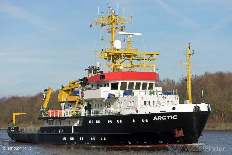
The experiment was conducted by the vessel MV “Arctic” (Figure 3), a 51 m long vessel chartered by Aker BP to conduct a seismic survey in the North Sea.
Figure 3. MV "Arctic".
2.2 - Sound source
A sparker source generates sound by discharging high-voltage electrical current from a bank of storage capacitors. A sparker is a seismic source that uses an electrical discharge from a ship-based power supply (100s to 10,000 J) to vaporize saltwater, rapidly creating a bubble that produces an omnidirectional pulse of sound, typically up to 3 ms in duration and with most energy between 50 Hz and 4 kHz (BOEM, 2023).
The frequency range of a sparker source is thus higher than for both seismic air guns and marine vibrators, and with lower power, usually with a source level of 185-226 dB 1µPa @ 1m (Ruppel et al. 2022). The pulse repetition rate is short, usually 0.25 s, hence almost acts as continuous source.
The sparker source is relatively easy to deploy and uses low power. It cannot be used to image deep targets, but is typically used for high resolution seafloor imaging prior to windfarm installations.
The sparker source used in the current study is shown in Figure 4. Two of these pictured sources were used together during the sparker treatments.
Figure 4. The sparker source used in the current study (photo: Kate McQueen). Two such sources were used together for the sparker treatments.
2.3 - Hydrophones
The two hydrophone rigs each had two types of hydrophones; a Naxys hydrophone and a sound trap. They were rigged as shown in Figure 5 and described in detail below.
Figure 5. Hydrophone setup. Left: Picture of the Naxys and sound trap hydrophone and the PC for the Naxys hydrophone. Right: Rigging of hydrophones. The hydrophones are deployed 8 m above the seafloor, and held down by a weight of about 30 kg. An underwater float is mounted on the rope 30 m above the hydrophone to keep the rope stretched out. A surface bouy marks its position at the surface.
2.3.1 - Naxys Ethernet hydrophones
Naxys 02345 Ethernet Hydrophones are omni directional, with a frequency range of 5 Hz to 300 kHz, and a sensitivity of -179 dB re V/µPa. They were programmed to record sound pressure at 23 s intervals with 1 s pauses, and 48 kHz sampling rate was used. The hydrophones have an amplifier with an adjustable gain from 0 to 40 dB, and 40 dB gain was used. All hydrophones were calibrated before the survey using a Brüel & Kjær 4229 piston calibrator. RBR depth loggers were attached to each hydrophone to record their depths and vertical movements during the survey. Specifications of the hydrophones are given in Table 1.
Table 1. Naxys Ethernet hydrophone 02345 specifications (serial Nr 02,03,04 and 05).
Parameter
Value
Units
Hydrophone sensitivity
-179
dB rel V/µPa
Element sensitivity
-211
dB rel V/µPa
Frequency range
5-300k
Hz
Sensitivity accuracy
+/- 3
dB
Pattern
Omni directional
The battery capacity of the Naxys hydrophones allow 1-2 days of recording, and in previous experiments their performance has been a bit unstable, so therefore recovery of both rigs was planned after block 2 to charge the battery and check that they did actually record as planned.
2.3.2 - Sound trap hydrophones
The sound trap hydrophone was of type STD 300 from Ocean Sonics. The purpose of this was dual; to record cod vocalisations in the area, and to act as back up for recording the sparker/vessel sounds in case the Naxys hydrophones failed.
2.3.3 - Calculations of sound pressure levels
The data were calibrated with a Brüel & Kjær 4229 piston calibrator with a specially made coupler. The rms level for the Naxys hydrophones in the special coupler should be 148.5 dB re 1 uPa. A calibration factor was estimated for each of the hydrophones based on this. The sampling interval was 22 sec recording, 8 sec break.
The sound trap hydrophones are factory calibrated. The standard factory calibration consists of a piston phone calibration and are accessible online throughout the calibration page of the Ocean Instruments website (http://www.oceaninstruments.co.nz/) by inserting the hydrophone serial number. For more details see (https://www.oceaninstruments.co.nz/wp-content/uploads/2015/04/ST-User-Guide.pdf). The calibration should be applied to the data with fullscale signal within ± 1. That is the maximum measurable values are within ± 1. To achieve this, the signal should be normalized by dynamic range. The dynamic range, DR, is related to the bit depth (BD) as DR as DR=2BD . Therefore the raw data should be divided by 0.5 DR and multiplied by the calibration factor. The calibrated data has unit of µPa. The calibration factor is estimated as 10Gain(dB)/20 .
The sound trap hydrophone records continuously with the sample rate of 48 kHz.
Sound Exposure level (SEL) was estimated using 10 seconds signal duration throughout each 2 hour treatment.
2.4 - Hydrographic measures
A Conductivity-Temperature-Depth (CTD) instrument was used to make a profile of the temperature of the water column. This allows calculation of a sound speed profile in the area as well as locating the depth of sound channels. A SAIV SD204 ( Figure 6) was used.
Figure 6. The SAIV 204SD CTS sonde being lowered into the water.
2.5 - Exposure design
The experiment was conducted as a block design; each block consisting of three treatments; “sparker”, “vessel noise” and “silent”.
The “sparker” treatment used the source with the same rigging as during an operational survey. The level was however initially set lower than during an operational survey, and gradually increased to pinpoint a potential level where the fish may react. Furthermore, we needed to be sure of the welfare of both the wild fish as well as farmed salmon in the area around. Therefore a 3-step level increase was planned; the first 2 blocks at the lowest level, the next 2 blocks at medium level and the remaining blocks at the level used in an operational setting. Source level 1 had a power level of 400J, source level 2 had a power level of 600J, and source level 3 had a power level of 800J. Source level 3 corresponded to the level used in the ongoing operational survey with this source, hence the level to be experienced in a real operation. During the sparker treatments, the sparker source was turned off as the vessel made the turns at either end of the racetrack (ca. 5 mins). This was to protect the equipment and mimic normal operational activity.
During the “vessel noise” treatment, the vessel transited the exact same racetrack as for the sparker treatment, but without deploying the sparker. The reason for this is to be able to separate any reactions to the sparker sound from just the vessel sound.
During the “silent” treatment, the vessel left the area for a place where the vessel would be outside the hearing range of the fish; hence without causing any disturbance, acting as a control.
Each block lasted 2 hours. The blocks and treatments within the blocks were randomly generated. A treatment schedule of 9 blocks was made prior to the experiment, and we aimed to conduct as many of these as possible. These are shown in Table 2 .
Block
Run
Treatement
Sparker Level
1
1
sparker
1
1
2
vessel
1
3
silent
2
1
vessel
2
2
sparker
1
2
3
silent
3
1
vessel
3
2
silent
3
3
sparker
2
4
1
vessel
4
2
sparker
2
4
3
silent
5
1
silent
5
2
sparker
3
5
3
vessel
6
1
vessel
6
2
sparker
3
6
3
silent
7
1
silent
7
2
vessel
7
3
sparker
3
8
1
vessel
8
2
sparker
3
8
3
silent
9
1
vessel
9
2
silent
9
3
sparker
3
Table 2 . Planned treatement schedule
2.6 - Fish farms
The area in Austevoll where the experiment was conducted is an area that also has fish farms around. We therefore contacted all nearby fish farms to inform them about the experiment. For the closest fish farm, we were in close contact throughout the entire operation, and always informed them about the starting time before we started transmission, so that they could monitor the fish and alarm us if any sign of unwanted behavioral response was observed (e.g. fish startle and swim to bottom of net pen). If such responses were to occur, we would stop the operation immediately. However, no abnormal behavior was reported, even at the highest sound level. This fish farm is located about 1.5 km from the closest point of the racetrack.
3 - Results
The experiment was conducted from May 27th to 29th 2023. The survey was a sudden opportunity offered by Aker BP as the ship was in Bergen waiting for better weather in an ongoing operation in the North Sea. Since the opportunity arose so suddenly, all clearances, permissions and logistics needed to be organized very quickly to enable to survey to take place. Since the vessel was foreign (from the Netherlands) we additionally needed a permission from the Norwegian Armed Forces to operate in coastal waters, and this delayed the survey for about a day to wait for clearance. Further, the weather improved quicker than expected, hence we needed to break off a bit earlier than first planned. Additionally, deployment and retrieval of the hydrophone rigs took more time than expected. Therefore, we only managed to conduct 6 of the planned 9 blocks. The first two were of source level 1, and since we aimed to have at least two blocks with level 3, the second level 2 block was dropped. Further, to get most out of the available ship time, the silent treatment of block 5 and the vessel treatment of block 6 were dropped. This decision was made as we already had several replicates of silent and vessel treatments, and to maximise the number of replicate sparker treatments within the limited survey period.
The final treatment schedule is shown in Table 3 .
Block
Run
type
Source level
Start date (local)
Start time (local)
Stop time (local)
1
1
sparker
1
27.05.2023
22:25
00:25
1
2
vessel
28.05.2023
00:25
02:25
1
3
silent
28.05.2023
02:25
04:25
2
1
vessel
28.05.2023
04:25
06:25
2
2
sparker
1
28.05.2023
06:25
08:25
2
3
silent
28.05.2023
11:00
13:00
3
1
vessel
28.05.2023
13:50
15:50
3
2
silent
28.05.2023
16:05
18:05
3
3
sparker
2
28.05.2023
19:45
21:45
4
1
vessel
28.05.2023
21:45
23:45
4
2
sparker
3
28.05.2023
23:45
01:39
4
3
silent
29.05.2023
01:40
03:40
5
1
silent
5
2
sparker
3
29.05.2023
03:50
05:45
5
3
vessel
29.05.2023
05:45
07:49
6
1
vessel
6
2
sparker
3
29.05.2023
07:49
09:48
6
3
silent
29.05.2023
10:00
12:00
Table 3. Overview of the treatements conducted. Due to time constrains, one vessel control (block 6.1) and one silent control (block 5.1) was cacelled, indicated as deleted in the table.
3.1 - Hydrophone recordings
The hydrophone rigs were deployed and retrieved from the source vessel. This was however quite complicated and more time consuming than expected. Both rigs were recovered after block 2.2, since after this, there were 3 runs (6 hours) until the next sparker treatment that needed to be recorded, hence allowing time to recharge batteries during these runs (2 silent runs, 1 vessel run).
After retrieving the hydrophones, data was downloaded. It turned out that one of the hydrophones; serial number 005, placed in the outer position, had not recorded any data. This was therefore changed to serial 019 during the second deployment. Further the data on the other hydrophone appeared a bit strange. The gain was too low, and therefore the dynamic range was too high for digitization of the measured signal. Therefore, the gain was adjusted to hopefully improve this during the next recording. Additionally, the locations of the hydrophone rigs were switched between deployments, so that the rig that had been deployed in the inner bay during the blocks1.1-2.2 was moved to the outer bay for blocks 3.3-6.3, and vice versa.
The timing of the files recorded by Soundtrap refer to the local time (+2 UTC). The computer time of the Naxy hydrophones was 112 minutes behind the local time. This applies to the time of the files and was corrected when plotting the recorded signals.
The hydrophone deployments are shown in Table 4 .
Deployment Number
Hydrophone
Serial number
StartTime (local)
StopTime (local)
LAT
LON
Comment
D1
Bunnhydrofon 1 (BH1)
005
27.05.2023 20:16
28.05.2023 10:20
60.121299
5.071893
Deployed at inner bay location
D2
Sound trap 5513
5513
27.05.2023 20:16
28.05.2023 10:20
60.121299
5.071893
Deployed together with BH1 at inner bay location
D3
Bunnhydrofon 2 (BH2)
003
27.05.2023 20:20
28.05.2023 09:33
60.120335
5.09723373
Deployed at outer bay location
D4
Sound trap 5779
5779
27.05.2023 20:20
28.05.2023 09:33
60.120335
5.09723373
Deployed together with BH2 at outer position
D5
Bunnhydrofon 2 (BH2)
003
28.05.2023 16:47
30.05.2023 09:36
60.1212328
5.070824028
Deployed at inner bay location
D6
Sound trap 5779
5779
28.05.2023 16:47
30.05.2023 09:36
60.1212328
5.070824028
Deployed together with BH2 at inner position
D7
Bunnhydrofon 1 (BH1) *
019
28.05.2023 17:20
30.05.2023 09:57
60.1199634
5.095290887
Deployed at outer bay location
D8
Sound trap 5513
5513
28.05.2023 17:20
30.05.2023 09:57
60.1199634
5.095290887
Deployed together with BH1 at outer bay location
Table 4 . Overview of the hydrophone deployments. Note that the position of the two hydrophone rigs are swiched between the two deployments. This was done due to repeated failure of the two hydrophones.
* Hydrohone was changed due to undesired performance of Hydrophone with serial number 019.
3.1.1 - Sound characteristics and levels
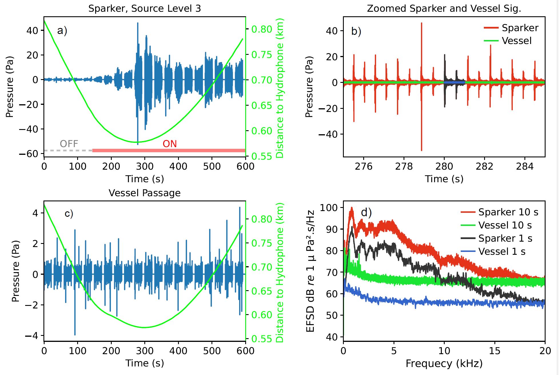
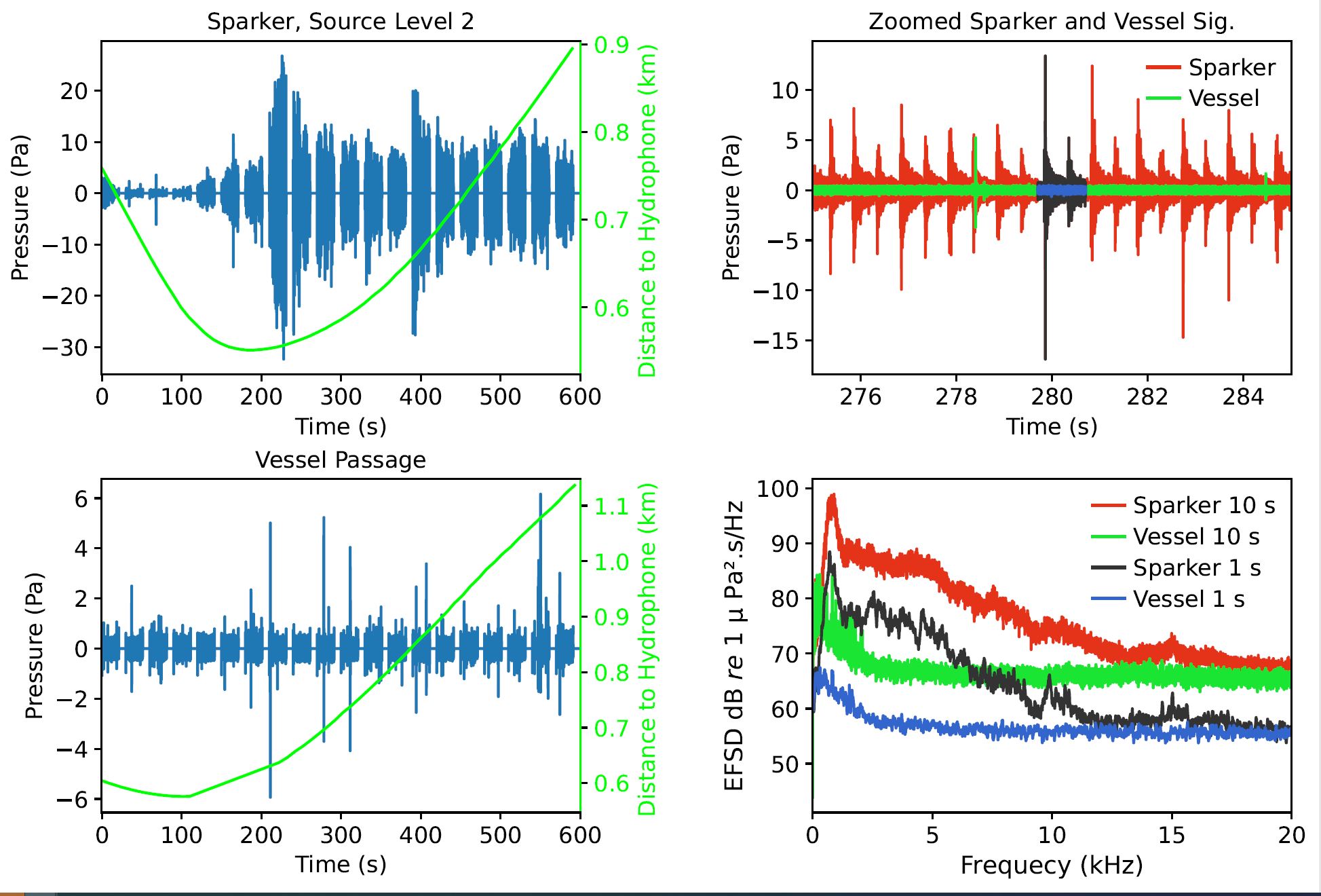
The sound signals from the sparker source are shown in Figure 7-10. The signal was ramped up at the start before reaching full power (Figure 7a). The sparker signal was clearly stronger than the vessel noise ( Figure 7 c). The sparker signal has energy from a few Hz and up to at least 10 kHz, with a peak around 1 kHz ( Figure 7 d and Figure 8 d).
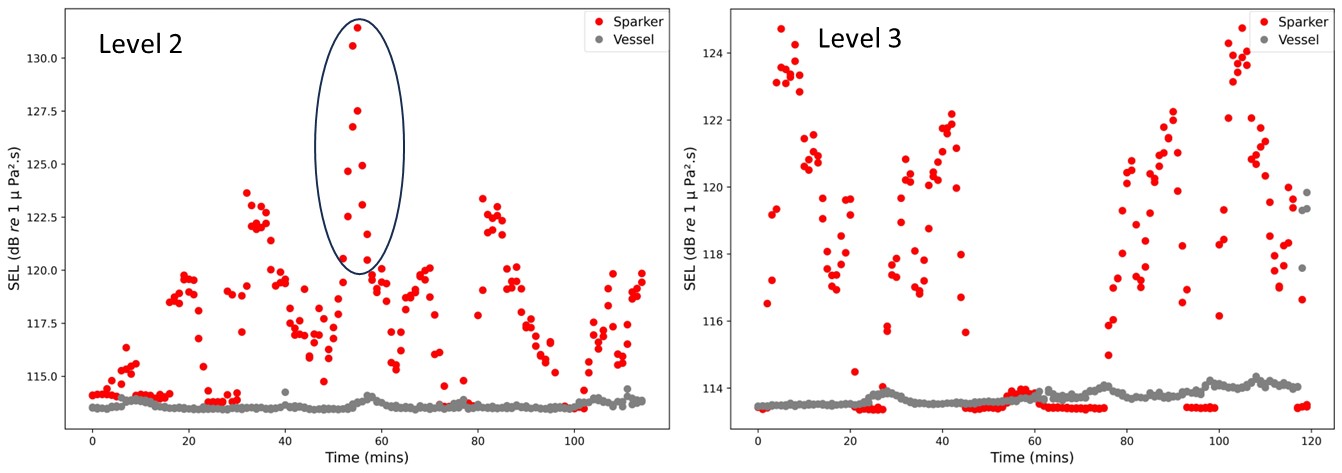
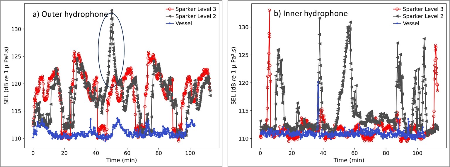
The sound exposure level, integrated over 10 sec, at the outer hydrophone was approximately 125 and 123 dB re 1µPa2 s, for levels 3 and 2, respectively (Figure 11). At the inner hydrophone, the signal from the sparker was not clearly detectable above the vessel noise. This hydrophone was placed in an area with many cottages around and with the survey conducted on a long-weekend (public holyday) in May, there were quite a lot of recreational boats around. This made it challenging to extract purely the sparker signal for the duration of a full treatment period, as can be seen in Figure 13 .
The sparker signal was sent as a “spark” every 0.5 seconds for the full exposure duration, hence leaving only very minor gaps between each signal.
Figure 7. Overview of the recorded sound signals from the outer hydrophone at level 3 (loudest signal). a) and b) show the sound pressure as a function of distance and time for the sparker signal (a) and vessel passage (b). c) is zoomed in for a period of 10 sec, showing the single sparks in more detail. The red/black and green/blue in c) corresponds to the red/black and green/blue in d) showing the Energy Flux Spectral Density (EFSD) over 10 sec (red and green for sparker and vessel, respectively) and for 1 sec (black and blue for sparker and vessel, respectively). The figure show recordings from the outer hydrophone position (see location in Figure 1) recorded by the Naxys hydrophone.
Figure 8. SImilar as Fig. 7, but for level 2 source level.
Figure 9. Energy flux spectral density recorded by the sound trap for a) several individual sparker signals (shown in different colours) and b) a same duration time period without the sparker signal (silent treatment). As can be seen in a), the sparker signal have energy over the full frequency spectre up to 10 kHz, with a peak around 1 kHz. Please note that these levels are not calibrated.
Figure 10. High-passed filtered Recordings by the outer sound trap hydrophone. a) show the sailing track for the measured sound level in b). The vessel is approaching the bay, sailing direction indicated by the arrow, ending up with the marked red circle. In b) the sound signal can be seen as increasing as the sparker is starting transmitting at time = 300, and reaching maximum as the hydrophone position is passed and then decreasing as the vessel moves away. In c) a 10 sec time period is zoomed in to see the individual signals. As can be seen here, one signal is transmitted every second. d) Same duration as for b) for the inner hydrophone, showing that the sparker signal here is not detectable above the background noise level.
Figure 11. Sound Exposure Level (SEL) for the sparker source at the two highest levels throughout a full 2 hour exposure run recorded at the outer hydrophone. Note that for level 2, the peak in the middle (points inside circle) is not attributed to the sparker, but to a vessel passing close to the hydrophone, see also figure 12 for details of this. For level 3, those points clearly lying at the same level as the ship noise are from the turns (“corners”) of the racetrack, when the source was turned off. These measurements are from block 3 (Level 2) and block 4 (Level 3).
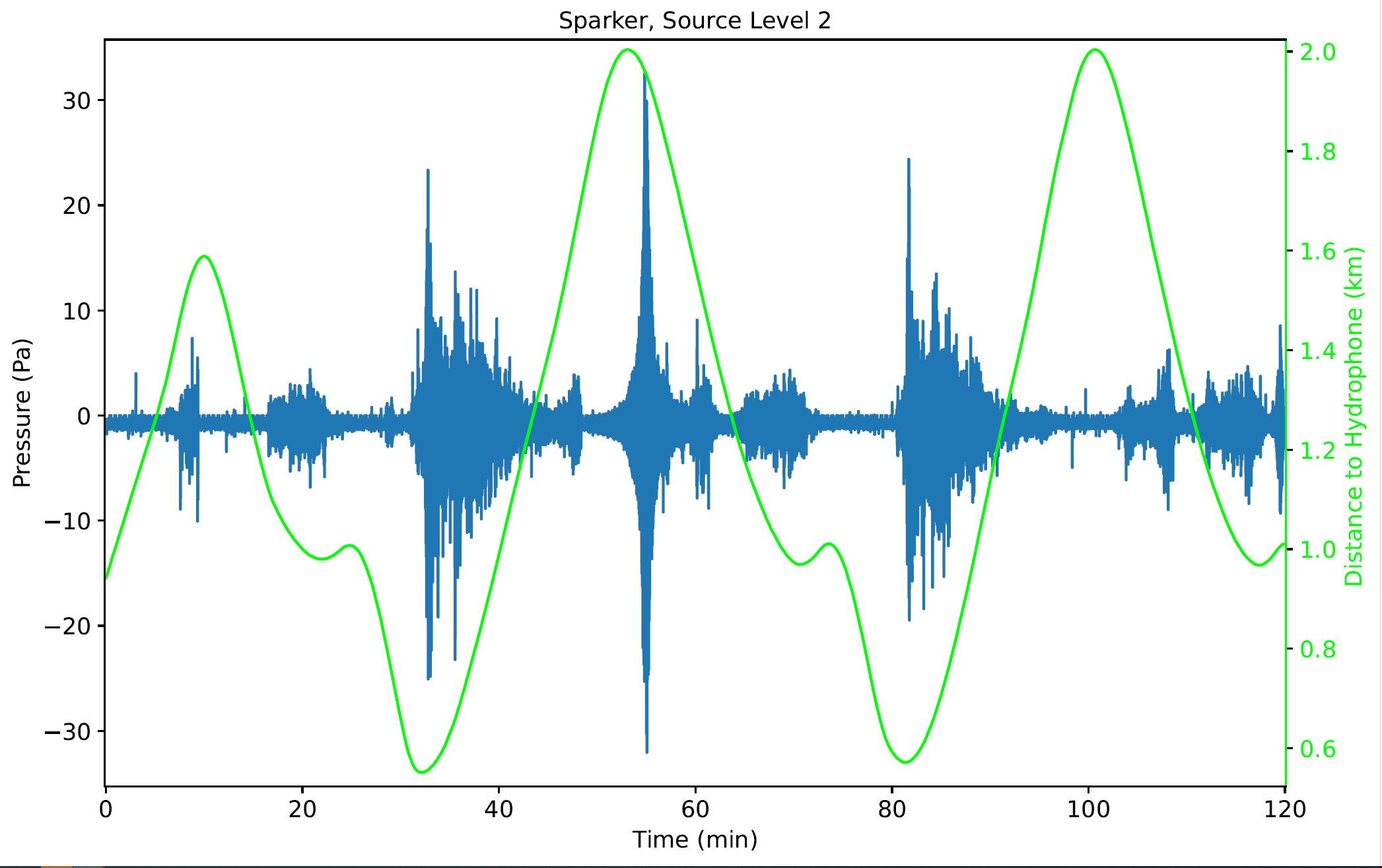
Figure 12. Pressure signal (blue) and distance from hydrophone (green) for the level 2 signal data for the calculations resulting in the plot in figure 5. As can be seen, at time around 52-57 min from start, there is a clear peak at a time when the source vessel is at the furthest distance. The level from the source should hence be similar as for time around 100 min after start, hence when the ship was at the same position during the second round around the race track. Therefore, the peak seen here are not from the sparker source, but rather likely from a boat passing close to the hydrophone.
Figure 13. SEL over 10 sec from outer Sound trap hydrophone (a) and inner sound trap hydrophone (b) for the two sparker levels 2 and 3 and the vessel treatment. The data for the vessel and sparker treatments are from block 4, starting at 21:45:00 and 23:45:00, respectively, while sparker level 2 are from block 3, starting at 19:45:00. The high peaks for level 2 seen both in the outer (indicated by a circle), in in particular for the inner bay, are likely from recreational boats passing the hydrophone rather than from the sparker signal.
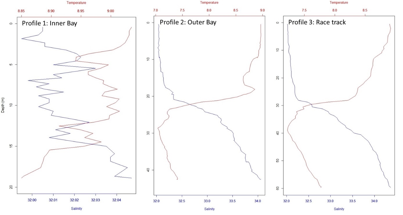
3.2 - CTD recordings
A total of three CTD casts were taken, at the 2 hydrophone locations and at the racetrack ( Figure 14 ). The details are shown in Table 5, and CTD profiles are shown in Figure 15.
CTD cast number
Time (local)
Lat
Lon
Comment
1
27.05.23 20:56
60.122145
5.07043
near inner bay hydrophone position
2
27.05.23 21:32
60.12018
5.09839
near outer bay hydrophone position
3
28.05.23 13:43
60.11527
5.112239
Middle of racetrack
Table 5. Details of the CTD casts.
Figure 14. Map of the CTD cast locations.
Figure 15. CTD profiles from the 3 casts showing salinity (blue curves) and temperature (red curves) as a function of depth.
3.3 - Fish behaviour
The behavior of the fish during the exposure have not been fully examined yet, but analyses similar to those done for the seismic exposure (McQueen et al. 2022; 23) and marine vibrator exposure (McQueen and Sivle et al. 2024) will be conducted. Here we show some preliminary examples of the data from fish presence and behavior.
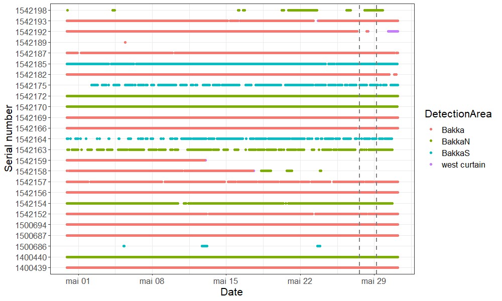
In total, 11 tagged cod were present in the test site throughout the experiment; 3 males, 4 females and 4 immature fish (sex not known). Additionally, 9 fish were detected either at the southern or northern gates of the telemetry grid (see Figure 1). The presence at the various sites throughout the month of May 2023 can be seen in Figure 16.
Figure 16. Presence of cod in the various receiver locations throughout May 2023. Fish ID refers to the individual tagged cod, and colored dots indicate that the fish was detected on one of the telemetry receivers in that area. The notations Bakka (red) is the main grid shown in Figure 1, while BakkaN (green), BakkaS (blue) and west curtain (purple) are the northern, southern and western gateways of the grid shown as D, E andC, respectively, in Figure 1. The grey stippled line indicates the period of the sparker survey.
Based on the first screening, there is no apparent drop in the number of fish present at the time of the sparker exposure period (28-30 May) as would have been expected if the fish were moving away from the habitat in response to the exposure. The general number of fish in the area was also similar as the previous years for the same time period ( Figure 17 ).
Figure 17. Number of fish present for day each day of May of the years 2019 – 2023. Shading indicates whether fish were classified as immature (Imm) or mature (Mat) at time of tagging.
Fish behavior will be analyzed with respect the swimming depth, activity level (acceleration) and movement inside the test site. No apparent change in swimming depth or activity level are seen in this first screening (Figure 18).
Figure 18. Acceleration in m s-2 (left) and swimming depth (right) of tagged cod during the periods of three types of exposure; silent, sparker and vessel treatment. These plots show all data for all individuals present in the test site, pooled together.
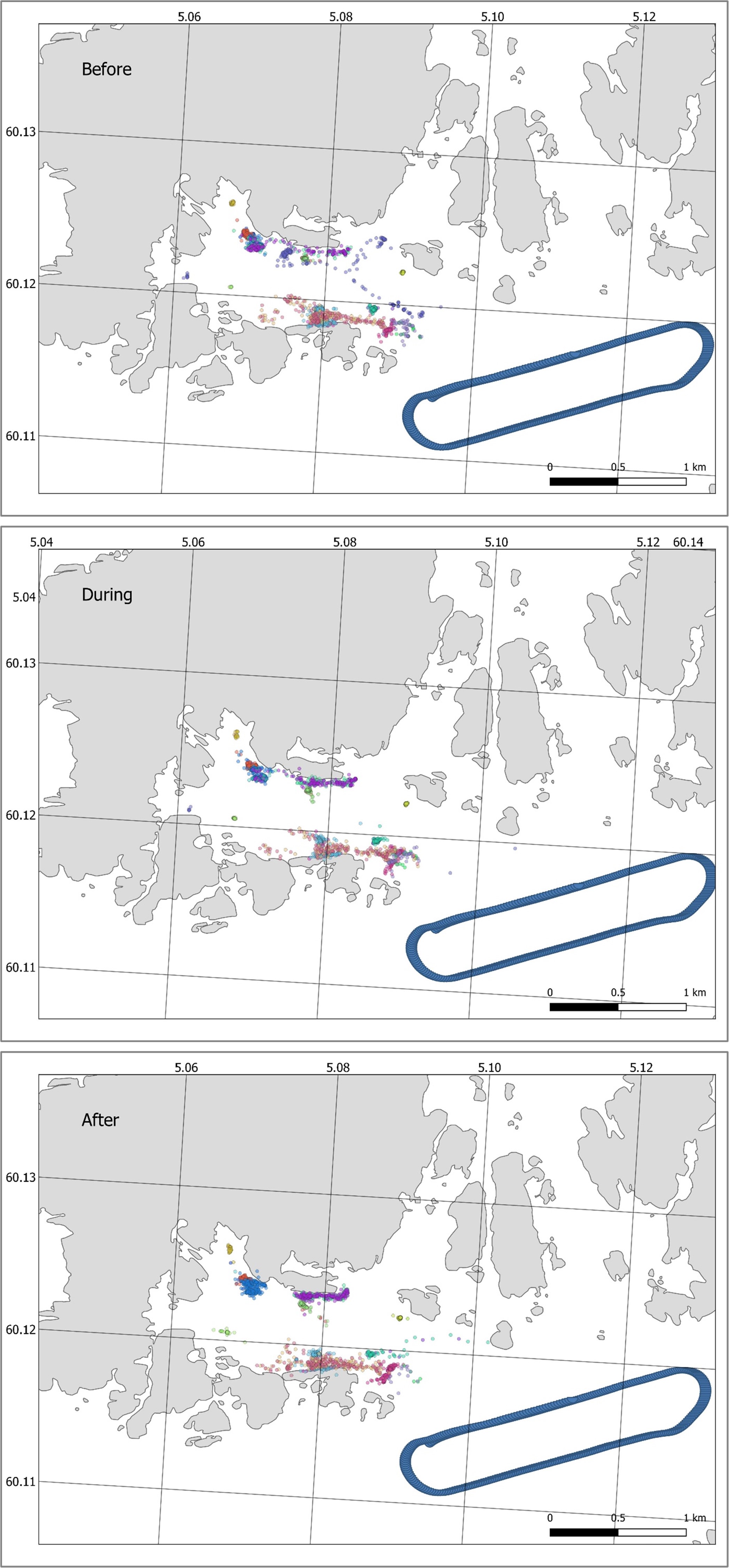
Observing the placement of the various fish inside the bay before, during and after the exposure (Figure 19) does not indicate any apparent change in distribution inside the bay attributed to the exposure.
Figure 19. Map showing the unfiltered positions of individual tagged cod in a similar time period before, during and after the exposure days. Each color represents an individual fish. “Before” period are from 25/05-2023 17:00 until 27/05 2023 09:00 UTC. “During” period are from 27/05.2023 17:00 until 09:00 UTC. “After” period are from 29./05 2023 17:00 until 31/05 2023 09:00 UTC. The location of the vessel racetrack is shown in blue.
4 - Data storage
All data collected in this survey are stored here:
The catalog structure follows that of most standard IMR surveys. Table 6 show the data structure and collected data.
Main folder
Subfolder 1
Subfolder 2
Description
PHYSICS
CTD
CTD data
MULTIMEDIA FILES
Photos
Photos taken during the survey. Folder for each phototgrapher
Videos
Videos taken during the survey. Folder for each phototgrapher
MAPS AND FIGURES
EXPERIMENTS
Hydrophones
soundtraps
Data from the sound trap recordings. One folder for each hydrophones.
Naxys
Data from the Naxys recordings. One folder for each of hydrophones.
Treatments
The final, executed treatment schedule
CRUISE LOG
Positions
Equipment
Files with positions for various important positions of the equipment
Ship Positions
Files with positions of the ship throughout the survey
CRUISE DOCUMENTS
Diverse tillatelser
Approved applications for survey
Notes
Notes taken during the survey
Table 6. Data structure and folder contents.
5 - Permissions
This survey was conducted with permission from the Norwegian Petroleum directorate to conduct a scientific survey, with permission number ( undersøkelsestillatelse) nr. 864/2023.
Permission to tag and conduct sound exposure with life fish was given by the Norwegian Food Security Authority (Mattilsynet), permission FOTS ID 29943.
Since the ship was a foreign ship operating inside the Norwegian territorial waters, an extra permission from the Norwegian Armed Forces was needed. This was given with the reference number 2023/001634-036/DFNON/414.
6 - Referances
Buogo, S., & Cannelli, G. B. (2002). Implosion of an underwater spark-generated bubble and acoustic energy evaluation using the Rayleigh model. The Journal of the Acoustical Society of America , 111 (6), 2594-2600.
BOEM, Center for Marine Acoustics (2023). Sound source list: a description of sounds commonly produced during ocean exploration and industrial activity. Sterling (VA): U.S. Department of the Interior, Bureau of Ocean Energy Management. 69 p. Report No.: BOEM OCS 2023-016.
Engås, A., Løkkeborg, S., Ona, E., & Soldal, A. V. (1996). Effects of seismic shooting on local abundance and catch rates of cod ((Gadus morhua) and haddock)(Melanogrammus aeglefinus). Canadian journal of fisheries and aquatic sciences , 53 (10), 2238-2249.
McQueen, K., Meager, J., Nyqvist, D., Skjæraasen, J.E., Olsen, E.M., Karlsen, Ø., Kvadsheim, P.H., Handegard, N.H., Forland, T.N. and Sivle, L.D. Spawning Atlantic cod (Gadus morhua L.) exposed to noise from seismic airguns do not abandon their spawning site. ICES Journal of Marine Science, 79(10), 2697-2708.
McQueen, K., Meager, J., Nyqvist, D., Skjæraasen, J.E., Olsen, E.M., Karlsen, Ø., Kvadsheim, P.H., Handegard, N.H., Forland, T.N. and Sivle, L.D. Behaviour of wild, spawning cod ( Gadus morhua L .) to seismic airgun exposure. ICES Journal of Marine Science, 80(4), 1052-1065
McQueen, K., Sivle, L.D., Forland, T.N., Meager, J.J., Skjæraasen, J.E., Olsen, E.M., Karlsen, Ø., Kvadsheim, P. and de Jong,K. (2024). Continuous sound from a marine vibrator causes behavioural responses of free-ranging, spawning Atlantic cod (Gadus morhua). Environmental Pollution, 123322, ISSN 0269-7491, https://doi.org/10.1016/j.envpol.2024.123322.
Sivle, L.D., Forland, T.N., deJong, K., McQueen, K., Schuster, E., Kvadsheim, P., Ektvedt, K.W., Aune, H., Laws, R. (2022). SpawnSeis MV exposure experiment – Survey Report – IMR survey number 2022812. Report series: Toktrapporter. ISSN: 1503-6294. https://www.hi.no/hi/nettrapporter/toktrapport-en-2023-4
Sivle, L.D., Forland, T.N., Handegard, N.O., Kvadsheim, P.H., Ektvedt, K.W., Schuster, E. and McQueen, K. (2021). SpawnSeis seismic exposure experiment on free-ranging, spawning cod. Toktrapport Nr 9-2021. ISSN: 1503-6294.
Ruppel, C. D., Weber, T. C., Staaterman, E. R., Labak, S. J., & Hart, P. E. (2022). Categorizing Active Marine Acoustic Sources Based on Their Potential to Affect Marine Animals. Journal of Marine Science and Engineering , 10 (9), 1278.
Soudijn, F. H. et al. (2020). Population-level effects of acoustic disturbance in Atlantic cod: a size-structured analysis based on energy budgets. Pro Royal Soc B , 287, 20200490 van der Knaap, I., Reubens, J., Thomas, L., Ainslie, M. A., Winter, H. V., Hubert, J., ... & Slabbekoorn, H. (2021). Effects of a seismic survey on movement of free-ranging Atlantic cod. Current Biology , 31 (7), 1555-1562.