The North Sea Ecosystem spring cruise (NSEC) has been run since 2010 by the Institute of Marine Research (IMR) as a multi-purpose survey. The cruise is usually performed in mid-April – mid-May to investigate the horizontal and vertical distributions of hydrography, chemistry, phytoplankton and zooplankton as well as fish eggs and fish larvae. The 2023 NSEC delivered data and samples to the following projects: - Climate and plankton in the North Sea and Skagerrak (IMR 14920), Early life history dynamics of North Sea fishes (IMR 14917), Monitoring of radioactivity in Norwegian waters (IMR 15595), Monitoring of environment and plankton in coastal waters (IMR 15593) and CoastRisk (15507-05).
The objectives of the North Sea Ecosystem Cruise 2023 were:
To sample pre-selected stations along standard transects for physical, chemical, and biological parameters in the Northern North Sea and Skagerrak (IMR 14920, IMR 14917, IMR 15593)
To map the abundance, distribution, and species composition of phytoplankton, microzooplankton, mesozooplankton, and early life stages of fish (eggs and larvae). (IMR 14920, IMR 14917)
To monitor radioactive contamination in Skagerrak (IMR 15595)
To acquire samples for the development of standard metabarcoding analysis in the plankton monitoring (IMR 14920, IMR 15507-05)
1.1 - Monitoring of plankton, biogeochemistry and hydrography in the North Sea and Skagerrak (IMR 14920)
The aim of the IMR monitoring project ¨Climate and plankton in the North Sea and Skagerrak¨ is, 1) to collect and analyze biological, chemical, and physical data to characterize and understand the causes of variability in the North Sea and Skagerrak at the seasonal, and inter annual scales, and 2) to provide multidisciplinary data sets that can be used to establish relationships among the biological, chemical, and physical variability. The monitoring activity includes one regional coverage per year (the spring survey in April/May) and additional sampling along three standard transects 4 times (Utsira-StartPoint, Hanstholm-Aberdeen and since 2021 Scotland East Coast and Fair Isle-Pentland) or 12 times per year (Torungen-Hirtshals).
The spring survey on plankton and hydrography in the North Sea - Skagerrak has been carried out by the institute of Marine Research since 2006. From 2006 to 2014, the survey was undertaken as a combination of two cruises running in parallel: The Environmental cruise" (Miljøtoktet on RV G.M. Dannevig) in the Skagerrak, and ¨The North Sea plankton survey¨ (usually on RV/ Johan Hjort) in the northern North Sea. In 2010, sampling of fish eggs and fish larvae was included in the sampling program, and the survey was renamed to The North Sea Ecosystem Cruise (NSEC). Since 2015, the former two spring surveys in Skagerrak and the North Sea have been combined into one single cruise, covering both the northern North Sea and the Skagerrak.
1.2 - Early life history dynamics of North Sea fishes (IMR 14917)
The Early life history dynamics of North Sea fishes project at IMR aims to determine the distribution and abundance of fish eggs and larvae in the northern North Sea and to link these observations to the biotic and abiotic environment. Depth integrated distribution of ichthyoplankton is provided by Gulf VII hauls alongside the sampling of zooplankton and oceanography. A Multinet Mammoth can be used to investigate the vertical and diel distribution of ichthyoplankton and their predators and prey fields.
1.3 - Monitoring of radioactivity in Norwegian waters (IMR 15595)
Water samples are collected by IMR once a year from Skagerrak, for analyses of radioactive contamination (cesium-137). This project contributes to the national monitoring program "Radioactivity in the Marine Environment (RAME)" which is coordinated by the Norwegian Radiation Protection Authority.
1.4 - Exploring Metabarcoding for Zooplankton monitoring (14920/15507-05)
In this pilot study, we explore the potential for applying an easily implemented metabarcoding component in the routine monitoring of marine plankton on IMR cruises. The key motivations for adopting metabarcoding in plankton monitoring are as follows:
Community analysis : Metabarcoding allows for a more comprehensive and accurate assessment of marine communities by identifying a wide range of species present in a larger number of samples than is possible to analyze visually.
Tracking invasive species : Metabarcoding provides a powerful tool for the early detection and tracking of invasive species, helping to inform management strategies.
Tracking biogeographic range shifts : Metabarcoding enables the detection of distribution ranges shifts in plankton populations, particularly within closely related congeners, contributing to our understanding of their ecological consequences.
Seasonal succession of species : Metabarcoding can offer a detailed and time-resolved view of these seasonal successions, particularly in seasonally restricted groups such as meroplankton, aiding in ecosystem modeling and management.
Prey composition for fish and other predators : plankton are a crucial food source for many marine species, including commercially valuable fish. Identifying the prey species can enhance our knowledge of predator-prey interactions and support fisheries management.
2 - Materials and Methods
North Sea Ecosystem Cruise JH2023206
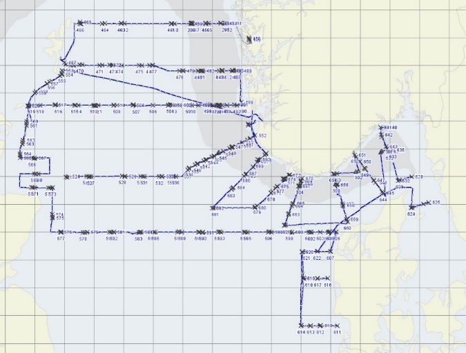
An overview of the total stations sampled during the North Sea Ecosystem cruise 2023 is presented in Figure 1.
Figure 1. Map of the stations sampled during the North Sea Ecosystem cruise 2023
A list of the personnel participating in the cruise, along with dates and their primary responsibilities, is presented in Table 1 while all the sampling equipment on board the ship is presented in Table 2.
Seawater temperature and salinity were measured at all stations with a SeaBird Electronics SBE911 CTD profiler fitted with a water bottle rosette.
2.2 - Biogeochemistry
Water samples for nutrient analysis (nitrate, nitrite, phosphate, silicate) were sampled from all CTD stations at all depths. From each depth 20 mL aliquots of sample water were collected in clean polyethylene bottles and added 0.2 mL chloroform, before storage at +4 ⁰C until further analysis at the Plankton Chemistry Laboratory at the Institute of Marine Research (IMR) in Bergen. Chlorophyll pigment samples (268 mL) were taken from eight depths between the surface and 100 m and collected on GF/F fiber glass filters. The filters were stored at -20 ⁰C to be analyzed for Chlorophyll- a and Phaeopigments (Chl- a , Phaeo) at the Plankton Chemistry Laboratory in Bergen.
2.3 - Phytoplankton
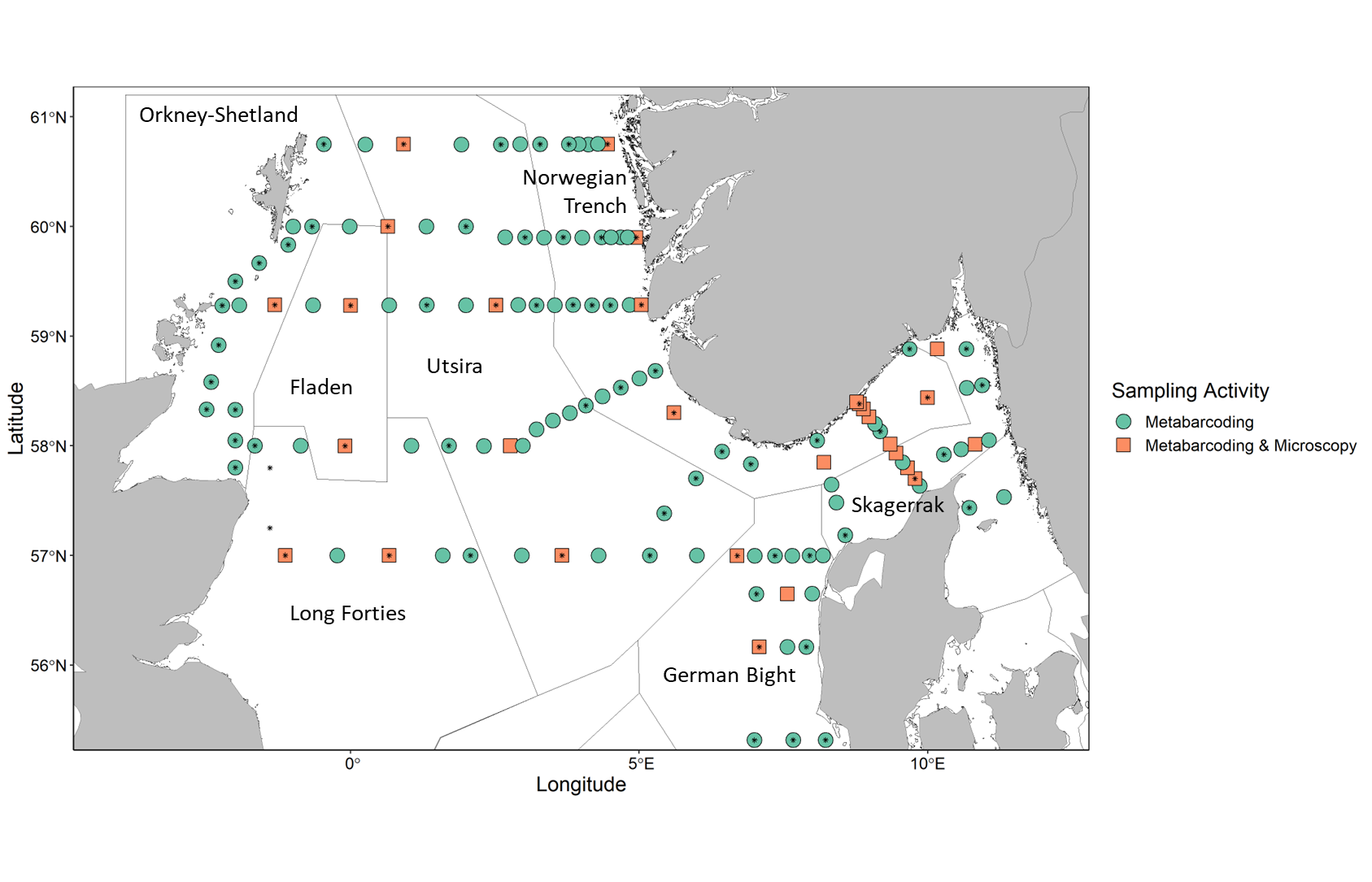
Samples used to characterize phytoplankton community composition and abundance were collected from a total of 131 stations. Microscopy was used to identify and quantify taxa in 29 preselected stations along the transects, covering multiple WGINOSE sub-regions (Figure 2). Algae-net and metabarcoding samples were also collected which can be used to qualitatively assess community composition. In total, 70 Algae-net and 129 metabarcoding samples were collected.
Samples for algal cell counts (100 ml) were taken from 10 m CTD collected water and fixed in Neutral Lugol. Microscope counts were performed following the Utermöhl (1958) method on CTD samples to quantify abundance and community composition at the Flødevigen Plankton Laboratory . Qualitative Algae-net samples were collected using a vertical net tow ( 10 μ m mesh; 0.1 m 2 opening; 30-0 m ), fixed with 2 ml 20% formalin and stored for future use. Metabarcoding samples were collected by filtering approximately 2000 ml of seawater, pre-filtered with 180 µm mesh, on to 25 mm filters with a pore size of 5 µm. Samples were then flash frozen in liquid nitrogen and stored at -80 °C for future DNA extraction and sequencing.
Microscopy algal counts include heterotrophic and autotrophic groups, these communities will therefore be referred to as microplankton in the summarized results below.
Figure 2. Map showing stations where phytoplankton samples were collected and analyzed. Shapes indicate sampling activities at a given station: circle- metabarcoding sample collection, square- microscopy sample analysis and metabarcoding sample collection, star: algae net sample collection. Outlined and labeled areas indicate WGINOSE sub-regions.
2.4 - Imaging Analysis of Plankton
Plankton samples for imaging analysis were collected at 63 selected stations along the standard North Sea transects. Samples were collected in parallel with phytoplankton and zooplankton microscopy samples to acquire a better understanding of North Sea plankton community structure. Water samples from microplankton enumeration, identification, and size structure analysis (500 ml) were collected from the 10m CTD sampler bottle, fixed in 2% (final conc.) acidic Lugol and stored in a dark refrigerated room (4 C). Samples for the zooplankton analysis were collected with a WPII and fixed with 4% formaldehyde. Post cruise analyses were performed at the Flødevigen Plankton Laboratory . Sampled were analyzed using a Flowcam VS-1 quipped with a 2x objective lens and a 800µm deep non-field-of-view flowcell (magnification = 20) , a flowcam 8400 laser equipped with a 10x objective lens and a 100µm deep field-of-view flowcell (magnification = 100), and a flowcam Macro with a 0.5x objective lens and a 5000µm deep field of view flowcell (magnification = 12).
2.5 - Zooplankton
Mesozooplankton were collected by vertical tows with WP-2 plankton nets (0.25 m 2 opening; 180 μm mesh size) from the bottom to the surface, and from 200-0 m, bottom depth permitting. Additional stratified sampling of zooplankton was carried out by Multinet MAMMOTH (Hydrobios, 180µm, 1 m 2 mouth opening, soft cod-ends). Oblique tows were made from 5 m above bottom while releasing nets at standard depths (Table 3).
Strata Depth
Multinet Number
0-bottom
0
bottom-400
1
400-300
2
300-200
3
200-150
4
150-100
5
100-50
6
50-25
7
25-0
8
Table 3. MultiNet standard depth of the IMR zooplankton monitoring in the North Sea-Skagerrak.
Large medusae and ctenophores were removed from whole samples, and the displacement volume of each species was recorded. The remaining zooplankton sample was split in two parts by a Motoda plankton splitter: one part was fixed in 4% borax buffered formaldehyde for species identification and enumeration. The other half was used for estimation of biomass (dry weight): samples were fractionated into three fractions (180-1000µm, 1000-2000µm and >2000µm) and placed on pre-weighted aluminum trays, dried at 60°C for 24 hours and kept in a freezer until return to Bergen. From the >2000 μm size fraction euphausiids, shrimps, amphipods, fish and fish larvae were counted, and their lengths measured separately before drying. In addition, Chaetognaths, Pareuchaeta sp. and Calanus hyperboreus from the >2000 μm size fraction were counted and dried separately (but sizes not measured).
Samples were not split on the transect Hanstholm-Aberdeen, due to shallow depths and small sampling volumes. Instead, two WP2-tows were taken: 1/1 sample was fixed in 4% formaldehyde, and 1/1 sample was fractionated and dried for later biomass measurements. All dry weights were determined at the IMR plankton laboratory in Bergen after the cruise. Details on the sampling procedures are found in the IMR Plankton Manual (Hassel et al., 2019).
2.6 - Macroplankton trawl
For the first time, the Macroplankton trawl was used on the NSEC to sample in the deeper regions of the Norwegian Trench. The aim was to obtain integrated samples of macroplankton from the Norwegian Trench for improved knowledge on the diversity and community structure of macroplankton and micronekton (>2 mm). The macroplankton trawl is a fine-meshed plankton trawl with an approximate 36 m 2 mouth opening and 3 mm stretched meshes from the trawl-opening to the rear end (Wenneck et al., 2008; Heino et al., 2011). The trawl was lowered vertically from surface to approx. 30 m above bottom and then hauled obliquely to the surface at ~2.5 knots.
Upon completion of trawl hauls the catches were weighed, and either the entire catch or a representative subsample was sorted. Species identification was made to the lowest possible taxonomic level, usually to genus or species level.
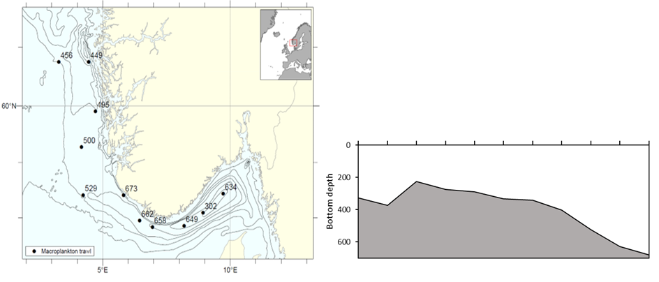
A total of 11 stations were completed with the Macroplankton trawl in the Norwegian trench (Figure 3a), along a transect following the bathymetry from Utsira in the north ( 60.750N; 3.280E) to the inner Skagerrak (58.446 N; 9.724 E). Trawl hauls were made at the deepest point in the trench, with bottom depth ranging from 226 to 680 m (Figure 3b). The oblique trawl hauls were made from 17 to 38 m above bottom, and maximum sampling depths of the trawl were 206 to 655m.
Figure 3. Macroplankton in the Norwegian Trench. Left) Stations sampled with the Macroplankton trawl (36 m 2 , 3 mm mesh, oblique hauls bottom-0m); Right) Bottom depth along the transect, ranging from 226 to 680 m.
2.7 - Ichthyoplankton
All GULF VII hauls were associated with a CTD station in close proximity. Temperature data in °C was extracted from the CTD records and used to interpolate temperature at 5 m depth, representing the surface layer, and for the lowest point of each CTD station, representing near-bottom temperatures. The interpolation was performed in R 4.3.2 (R Core Team 2023), using the autokrige function in the automap-package (Hiemstra et al. 2008).
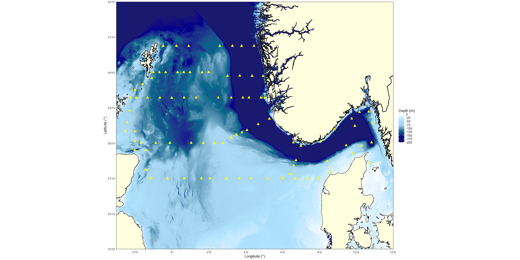
Ichthyoplankton was sampled with a Gulf VII high-speed sampler with a 76 cm frame and a 40 cm nose cone (Nash et al. 1998) at pre-determined stations along each of the standard transects (Figure 4). The net mounted on the GULF had a 280 μm mesh and a General Oceanics flow meter was fitted, slightly off center, in the nosecone, measuring the volume of water filtered. The sampler was deployed in double oblique hauls at 5 knots, down to a 100 m depth or within 10 m of the bottom. Fish eggs and larvae were sorted from the samples, or sub-samples thereof. Fish larvae were sorted into large taxonomical or functional (flatfish) groups, whilst the eggs were preserved pooled. Preservation was done in 4% seawater and Borax buffered formalin. A PUP sampler, equipped with a 5 cm diameter nosecone and a 80 μm mesh, was fitted on top of the GULF VII to provide samples of the fish larvae’s prey fields. Other than in previous years no flow meter was fitted to the PUP. PUP-samples were preserved in the same way as the GULF samples.
Figure 4. Executed GULF VII tows during the 2023 North Sea Ecosystem Survey. A total of 89 tows were conducted across the survey area. The underlying map shows the bathygraphy of the northern North Sea, with depths deeper than 200 m depicted in the same color.
To examine how the number and taxonomic composition of the larvae-samples relate to the abiotic environment we constructed a simple Generalized Linear Mixed Model (GLMM) in glmmTMB (Brooks et al. 2017), using taxonomic group, bottom depth, extracted from the 2023 GEBOC 15’’ grid (GEBCO Compilation Group 2023), and temperature as independent variables, with numbers raised to the complete sample as response and the filtered volume in m 3 as offset. Separate models were constructed for either surface or near-bottom temperature, with the other variables being the same. As there was a low number of zero stations a Gaussian probability distribution with an identity link was appropriate.
2.8 - Metabarcoding
Genetic samples were collected from 43 WPII net tows and 39 GULF VII net tows. A fraction of the sample, (typically ¼ for WPII, ½ for GULF VII) was rinsed with fresh water onto a sieve and transferred to the cup of a 1000W blender. The volume was topped up to 125 mL with MilliQ water and the sample was blended for ca. 1 minute until completely homogenous. 3 cryovials were filled with 4.5ml sample using a clean 5mL pipette tip and frozen at -20C. The remainder of the sample was discarded.In the laboratory, samples were thawed and centrifuged, and excess water was removed. Three replicates of 250 µL of the homogenate were transferred to a 96-well plate extraction plate and DNA was extracted using the Omega Blood and Tissue Kit using a Hamilton Microlab Star M robot according to the manufacturer’s protocol. The DNA was eluted in 50ul of elution buffer.
PCR and library prep followed protocols described in Ershova et al. 2022. All samples were sequenced on an Illumina Miseq using ¾ of a V3 2x300 Illumina flow cell.
Bioinformatics and taxonomic assignments were done according to Ershova et al. 2022. Only MOTU’s that matched to holo- or meroplanktic organisms and contributed a minimum of 100 sequence reads were retained in the final dataset. Extraction replicates were pooled in the final dataset.
2.9 - Radioactivity
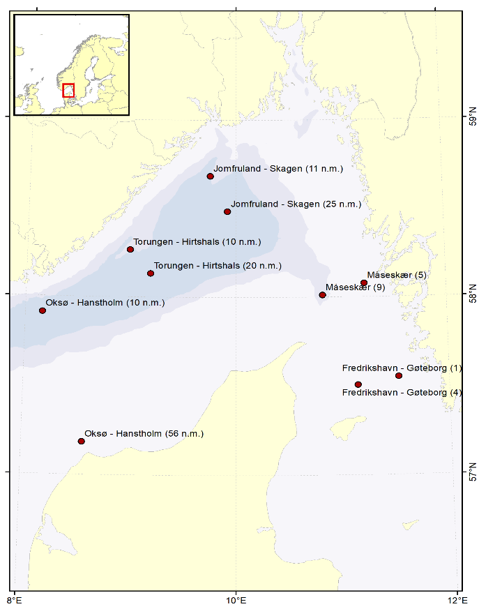
Water samples are collected yearly from 10 preselected stations in the Skagerrak (Table 4, Figure 5) for analyses of the radionuclide cesium-137 (Cs-137) (project number 15595). In 2023, sample collection was performed at 9 of 10 stations (Table 4). At each station, 50 liters of seawater are collected from the ship’s seawater intake and filled directly into 25 L plastic cans. The samples are later analysed for Cs-137 at the Laboratory for inorganic chemistry at IMR, Bergen, according to the internal method “460 - Bestemmelse av Cs-137 i sjøvann” (MET.UORG.01-17). This is a modified version of the analytical procedure described by Roos et al. (1994).
Transect
Station
Lat
Long
CTD station
Fredrikshavn - Gøteborg
1
57.55
E
11.53
N
Not collected
Fredrikshavn - Gøteborg
4
57.50
E
11.14
N
610
Måseskær
5
58.03
E
10.94
N
615
Måseskær
9
57.94
E
10.43
N
619
Jomfruland - Skagen (11 n.m.)
3
58.69
E
9.75
N
633
Jomfruland - Skagen (25 n.m.)
5
58.48
E
9.92
N
634
Torungen - Hirtshals (10 n.m.)
4
58.13
E
9.18
N
643
Torungen - Hirtshals (20 n.m.)
6
58.26
E
8.99
N
641
Oksø - Hanstholm (10 n.m.)
3
57.92
E
8.16
N
648
Oksø - Hanstholm (56 n.m.)
12
57.18
E
8.57
N
653
Table 4. Station list. Samples collected April 2023 for monitoring of Cs-137.
Figure 5 . Stations where seawater has been collected yearly since 2008 for analyses of Cs-137.
Monitoring of radioactive contamination in the Skagerrak is part of the national monitoring program Ra dioactivity in the M arine E nvironment (RAME), which is coordinated by the Norwegian Radiation and Nuclear Safety Authority (DSA) (e.g. Skjerdal et al., 2017; Skjerdal et al., 2020).
Transect
Station #
Nutrients
Chlorophyll a
Phytopl. Abund.
Phytopl. Net 30-0m
Phytopl. Metabarc.
Flowcam Micropl.
Zoopl. Metabarc.
WP2
WP3
Multinet
Gulf
Krill trowl
TOT NP
MIK
Fedje-Shetland
448-470
223
181
6
6
11
6
11
9
3
1
7
2
0
0
Slotterøy mot W
471-496
246
207
7
7
12
7
15
9
3
1
12
1
0
0
Utsira mot W
497-513
142
137
10
10
17
10
28
19
2
3
13
2
0
0
Jærens rev mot SW og W
514-537
204
183
7
8
16
8
25
15
2
3
13
1
0
0
Fair Isle - Pentland
538-350
82
95
6
6
6
6
12
6
0
0
6
0
0
0
Scotland East Coast
351-360
71
77
5
3
3
3
8
4
0
0
4
0
0
0
Hanstholm Aberdeen
561-587
149
176
8
10
15
8
14
21
4
3
12
0
19
Harboør
588-593
20
25
2
4
3
0
0
4
0
0
0
0
25
3
Knude dyp
594-601
25
33
3
3
3
0
0
4
0
0
0
0
25
3
Huseby klit
602-607
23
29
2
3
3
0
0
4
0
0
0
0
23
3
Gøteborg-Fredrikshavn
608-612
24
29
1
2
2
1
0
2
0
0
0
0
24
0
Måseskjær
613-620
68
64
1
4
3
2
0
2
0
1
2
0
40
0
Våderø
621-626
55
45
2
2
2
3
0
2
0
8
2
0
29
0
Jomfuland Koster
627-632
51
45
2
2
2
1
0
2
0
5
2
20
0
Jomfruland-Skagen
633-634
24
16
0
0
0
0
0
0
0
0
0
1
0
0
Torungen -Hirtshals
635-646
99
83
3
12
12
4
0
7
0
1
3
0
55
0
Oksøy-Hanstholmen
647-653
58
47
2
3
4
1
0
4
0
1
3
1
10
0
Lindsness
654-660
66
55
1
1
1
1
0
4
1
1
3
1
0
0
Lista mot SW
661-666
59
48
2
3
2
1
0
6
3
1
4
1
0
0
Egerøya mot SW
667-674
66
61
1
1
1
0
0
6
3
1
4
1
0
0
TOT
1755
1636
71
90
118
62
113
130
21
30
90
11
270
9
Table 5 . Summary of the overall samples collected on the transects covered by the North Sea Ecosystem Cruise 2023.
3 - Results
3.1 - Hydrography
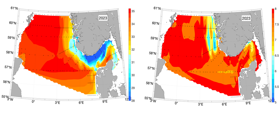
The hydrographic coverage of the survey area provides information on the main characteristics of the water masses in the northern North Sea and in the Skagerrak. The lowest surface salinities are typically found in the Skagerrak due to the Baltic outflow of low-saline waters through the Kattegat and the supplement of fresh water from local rivers along the Skagerrak coast. The resulting low-saline surface waters then follow the Norwegian coast westward out of the Skagerrak and northward along the coast, as the Norwegian Coastal Current (NCC). The shelf area in the northern North Sea is typically dominated by inflow of Atlantic water from the north (from the Tampen area) and from the west between the Orkneys and Shetland as the Fair Isle Current.
Figure 6. Salinity (left panel) and temperature (right panel, in o C) at 10m depth based on the hydrographic stations (marked with black dots) taken between 16/4 and 11/5 2023.
Based on the hydrographic measurements from the Ecosystem Cruise from April 16 to May 11, 2023, the NCC can be identified in the resulting surface salinity map in the areas with the minimum values (Figure 6, left panel, blue and yellow colors). The low-saline areas in the Skagerrak extend relatively far south towards Denmark, then indicating winds from the North and/or Northeast. We also see relatively low temperatures varying between 5.5-6.5o C in the NCC off the west coast of Norway, although the temperatures in the coastal areas off Agder (southern tip) is like what is observed in the northern and central North Sea (Figure 5, right panel).
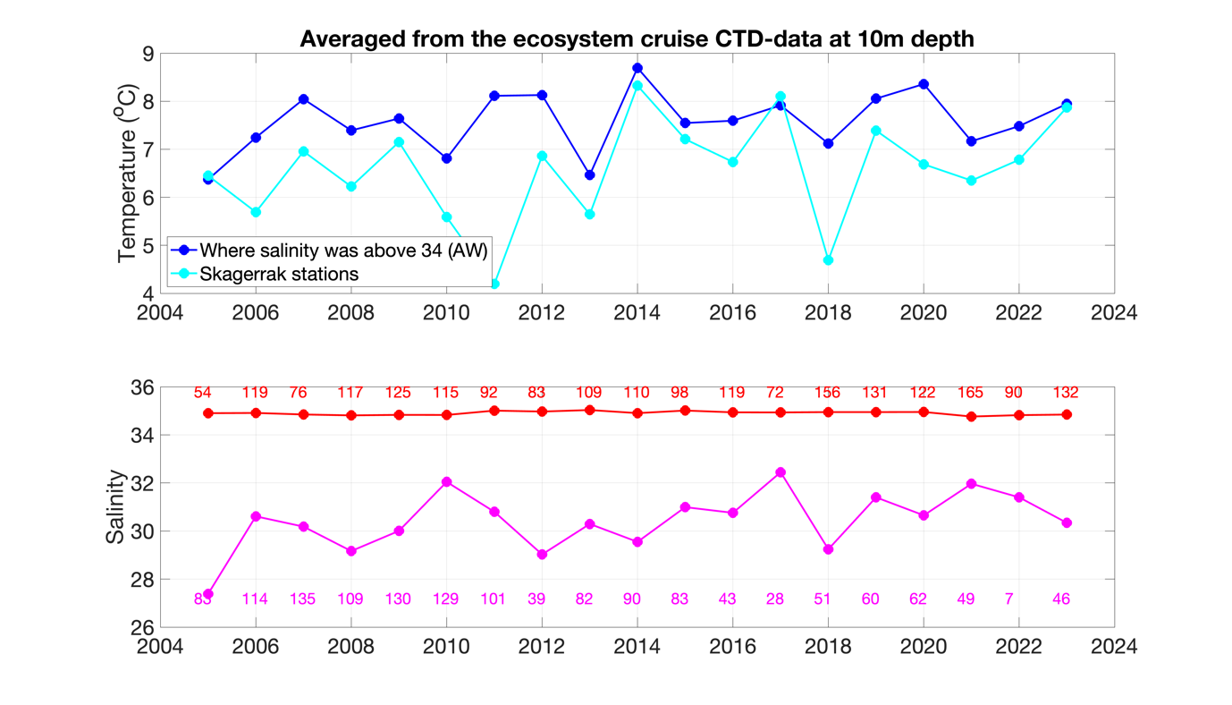
In relation to the long-term average based on all ecosystem cruises from 2005 until 2023, the Atlantic water in the northern North Sea and the Skagerrak waters were slightly warmer than normal in April/May 2023 (Figure 7). The temperature in both regions matched perfectly.
Figure 7. Time series of temperature (upper panel) and salinity (lower) at 10m depth as a spatial average over all ecosystem cruise stations for each year from 2005 to 2023. The stations have been separated in two categories: Areas heavily influenced by Atlantic water masses with salinity above 34 (blue and red) and Skagerrak stations (cyan and purple). Since the station coverage each year varies a lot, the number of valid data points is written as numbers in the lower panel.
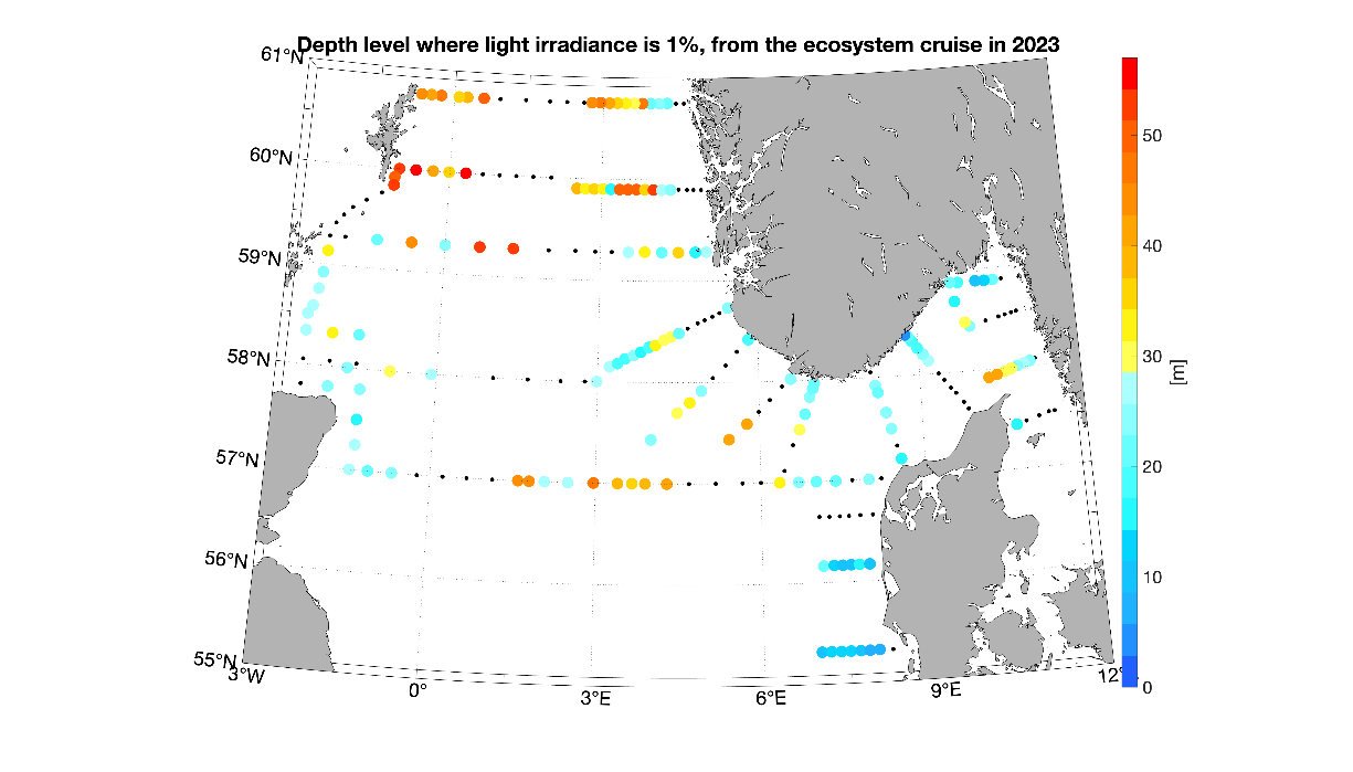
Photosynthetic organisms in the ocean, such as phytoplankton, use sunlight as their primary source of energy. Thus, they must live in the well-lit surface layer, the euphotic zone, to support the photosynthetic process. The light attenuation is an important parameter to determine the euphotic zone and can be influenced by the presence of both biotic and abiotic particles in the water. The depth of the 1% light irradiance gives an idea of the amount of particles in the water and the light available to phytoplankton. During the 2023 survey, the northern North Sea as well as the middle area of the Hanstholm-Aberdeen transect were characterized by the deepest 1% irradiance depth (Figure 8), suggesting a deeper mixed layer and low particles concentration. As matter of fact these areas correspond well with the lowest chlorophyll a concentration measured during our survey (Figure 9a).
Figure 8. Areal distribution of the 1% light irradiance depth. Warmer color indicates that light reached deeper layers and thus suggests lower particles concentration in the water.
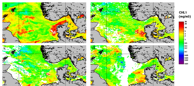
3.2 - Satellite image
Figure 9 shows the evolution of Chlorophyll a concentration in the studied area during the period April 15 to May 12. The images are mean values over 8-day period. The satellite images show higher accumulation of chlorophyll a along the coastal areas surrounding the North Sea. Specifically, during the first 8 days of the survey plums of high chlorophyll concentration were observed stretching from the coast of the United Kingdom towards the central area of the North Sea (Figure 9a). During the rest of the survey accumulation of chlorophyll a were observed mostly along the western coast of Denmark (Figure 9b, c, d).
Figure 9. 8 days mean surface chlorophyll-a concentrations over the survey period. a) 15-22.04; b) 23-30.04; c) 01-08.05; d) 09- 16.05. MODIS satellite.
3.3 - Biogeochemistry
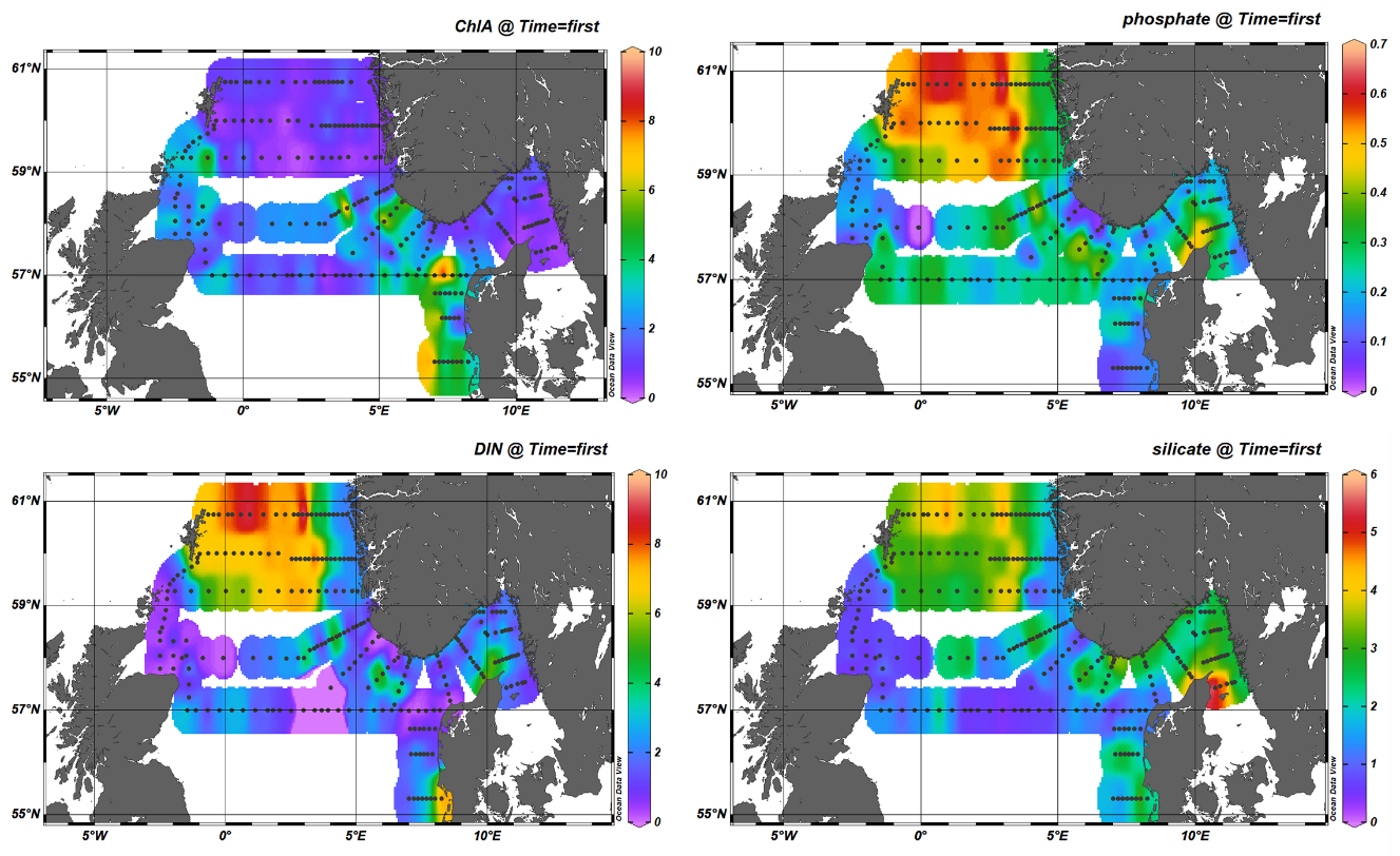
During the 2023 North Sea ecosystem survey chlorophyll a concentration ranged between 0.07 and 11.42 µg/L with the highest concentrations recorded along the west coast of Danmark (Figure 10a). In general, high chlorophyll a concentrations were associated with low nutrient availability suggesting previous use by phytoplankton. On the other hand, high total nitrate phosphate and silicate were measured in the Northwest sector (Figure 10b, c).
Figure 10. Chlorophyll a and nutrient concentrations during the North Sea spring survey 2023: Upper Left panel) Chlorophyll a; Upper Right panel) Phosphate; Lower Left panel) dissolved inorganic nitrogen ( DIN, nitrite + nitrate); Lower Right panel) silicate.
Silicate concentrations were usually high during our survey. Concentrations above 2μM were measured in the northwest sector as well as in Skagerrak. The highest value of 5.88 µM of silica was measured along the northeast coast of Danmark (Figure 10d). In general, 46% of the stations visited presented surface s ilicate concentrations <2μM. L ow silica concentrations are most likely the combined results of low initial values and/or previous diatom growth. Diatoms are in fact, the single user of silica, thus low values suggest a depletion of silica had occurred to fuel diatoms growth.
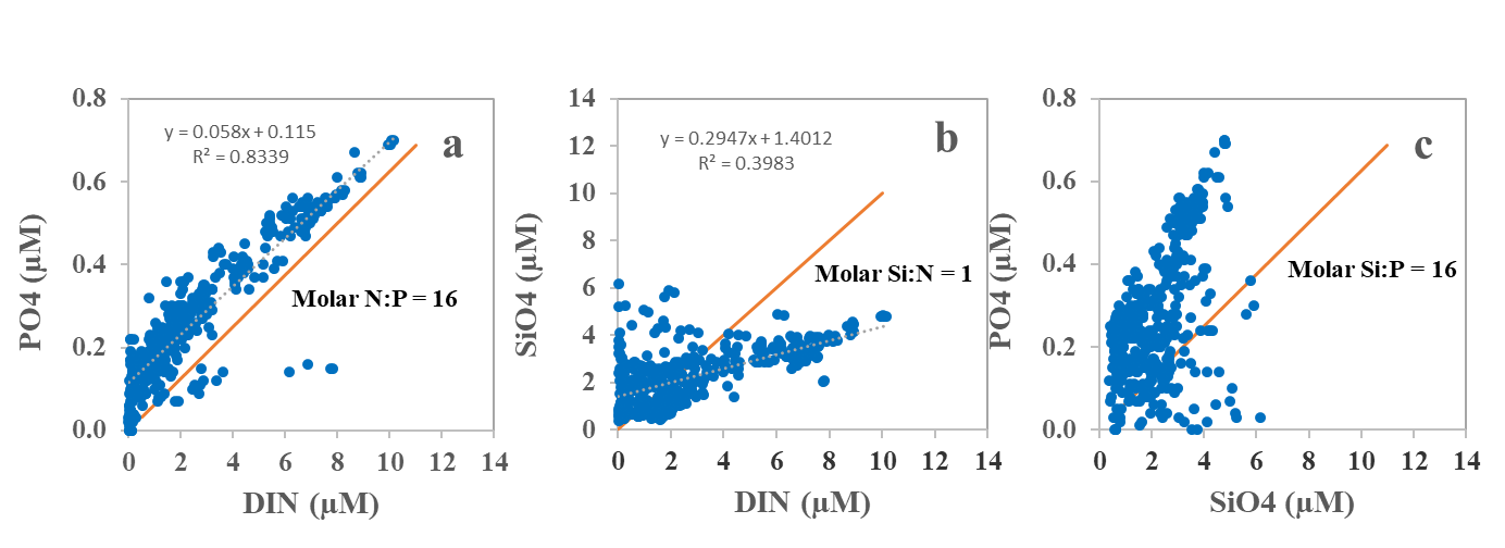
Overall, the station sampled during the 2023 survey showed an N:P-relationship lower than 16 for most parts of the North Sea (Figure 11) suggesting that phosphate was in abundance relative to DIN (nitrite + nitrate). Phytoplankton had less access to silicate than DIN, which may suggest that the primary producers were both silicate and nitrogen-limited (P>N>Si) in these areas.
Figure 11. Dissolved inorganic nutrients measured in surface waters (0-10 m depth). Phosphate (a) and silicate (b) were plotted as a function of dissolved, combined nitrogen (DIN= NO2+NO3), and phosphate (c) was plotted as a function of silicate. Whole line shows the Redfield N:P relationship and other molar relationships (N:Si, Si:P), necessary for a balanced cellular synthesis and growth in phytoplankton.
3.4 - Phytoplankton taxa
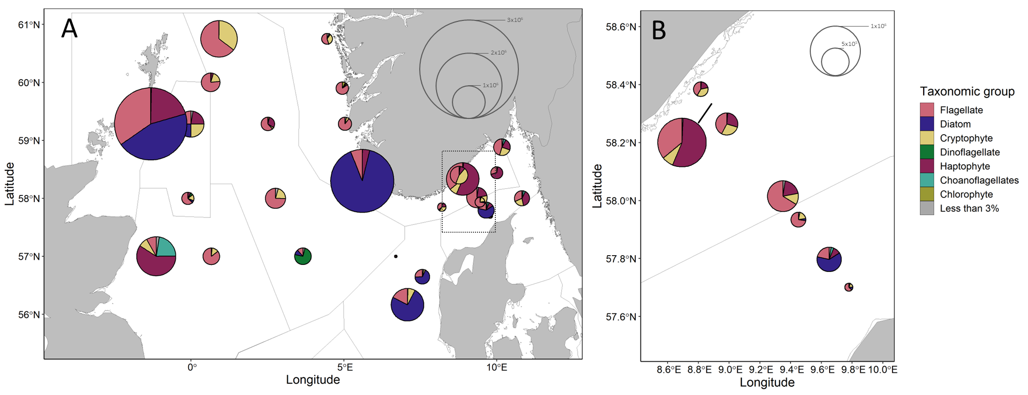
Based on microscopy counts, the North Sea microplankton community at an average station was numerically dominated by small flagellates (34%, 2.52×10⁵ ± 1.83×10⁵ cells L-1), diatoms (23%, 1.73×10⁵ ± 4.03×10⁵ cells L-1), haptophytes (18%, 1.34×10⁵ ± 1.86×10⁵ cells L-1) and cryptophytes (13%, 9.51×10⁴ ± 8.42×10⁴ cells L-1 ).
Microplankton abundances and communities varied spatially within the North Sea (Figure 12). Cell concentrations varied by more than an order of magnitude between stations, with a minimum concentration of 7.72×10⁴ cells L-1 and maximum of 2.22×10⁶ cells L-1 . Stations in the northern Norwegian Trench and central Utsira were characterized by low abundance communities composed mainly of flagellates and cryptophytes. Haptophytes, in addition to flagellates and cryptophytes, were abundant community members in the southern Norwegian trench and Skagerrak stations. Dinoflagellates were particularly abundant at a single station located in the south of the Utsira subregion, comprising more than 85% of the community. Diatoms comprised a large proportion of the community at only a few stations, most of which were located relatively close to a coastline.
Figure 12. Microplankton community composition and abundance. A) All sampled stations, B) Inset from map A showing Torungen-Hirtshals. Divisions within pie charts show the contributions from broad taxonomic groups in cells per liter. Pie chart radii scale to average cell concentrations. Groups accounting for less than 3% of a community at a given station are summed.
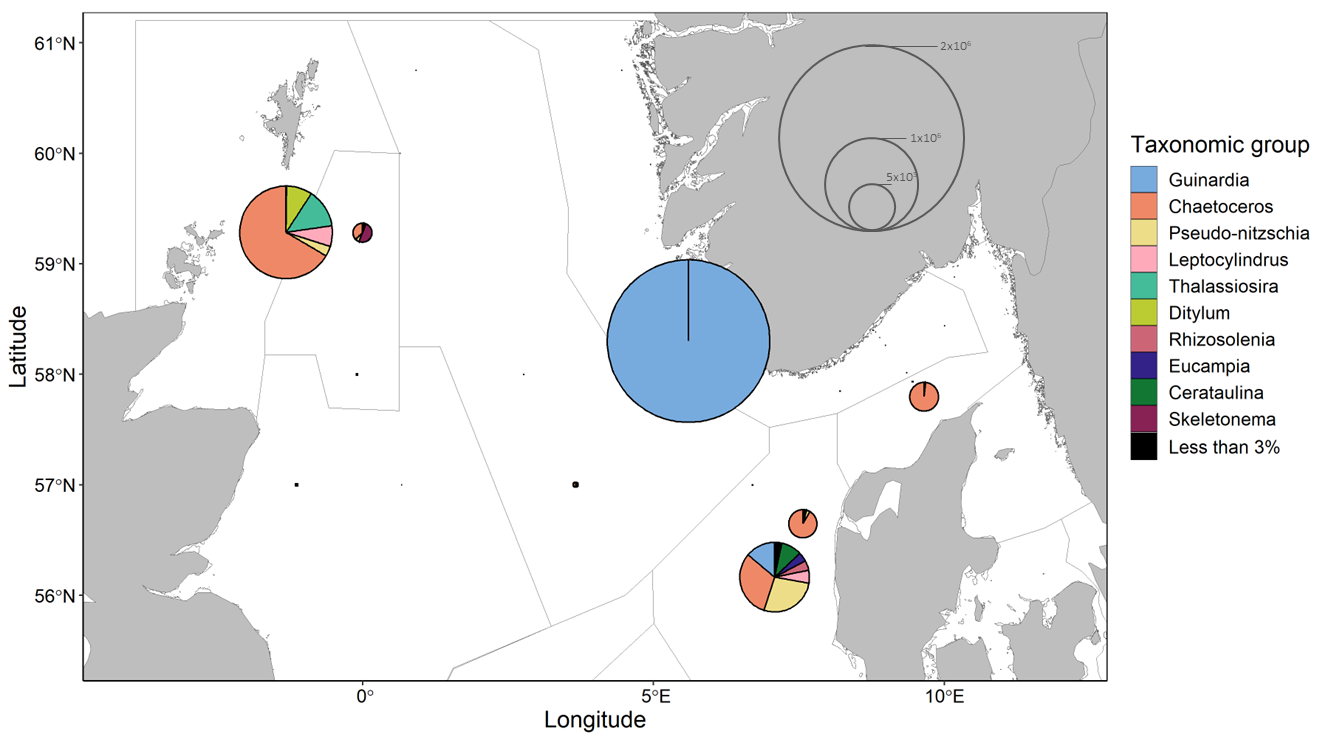
Within these data diatoms are the only purely photosynthetic group described at a high taxonomic level. Diatom abundance was greatest one station in the Norwegian trench where the diatom community was almost entirely comprised of Guinardia (Figure 13). At other stations where diatom abundances were greater than 1×10⁵ cells L-1, visualized in Figure 13, Chaetoceros comprised a large proportion of the community. Other taxa, such as Pseudo-nitzschia and Leptocylindrus, were also found at multiple stations where diatoms were relatively abundant.
Figure 13 . D iatom community composition and abundance at sampled stations. Pie chart radii scale to average cell concentrations. Divisions within pie charts show the contributions from different diatom genera in cells per liter. Groups accounting for less than 3% of a community at a given station are summed.
3.5 - Plankton through imaging analysis
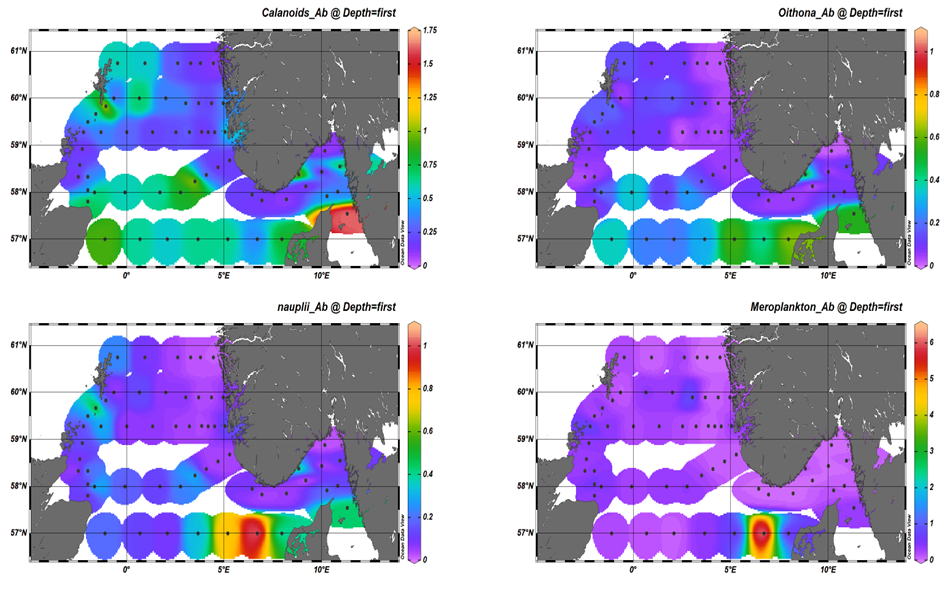
The analysis of microplankton is still underway. Here we focus on the flowcam analysis of the WPII samples. Through the imaging analysis of the larger component of plankton (>180 µm) we were able to distinguish several groups within the North Sea community. For reporting purpose, the groups were combined in: Calanoids, Oithona , Nauplii, Chaetognata, Euphausiacea, Appendicolaria, Meroplankton, and Others, which comprise both unidentified zooplankton and rare groups. During the 2023 survey, calanoids copepods were the most abundant group reaching 1.64 individuals per liter (Figure 14 a). Higher abundances were measured in the southwest sector of the North Sea as well as in the Skagerrak area. This result corresponds with the analysis microscopy (see following paragraph) which also reported large proportion of Calanus along the Aberdeen-Hanstholmen transect. Small copepods belonging to the genus Oithona , and nauplii were also quite abundant in our samples. Their abundances peaked at the eastern most stations of the Aberdeen-Hanstholmen transect (Figure 14 b,c). Worth of notice is also the high presence of meroplankton outside the west coast of Danmark were more than 6 larvae per liter were counted (Figure 14 d). As for the other groups their abundance was in general lower than 1 individual per liter.
Figure 14. Areal distribution of Upper Left panel) Calanoids copepod; Upper Right panel) Oithona spp., Lower Left panel) nauplii and Lower right panel) Meroplankton based on FlowCam imaging system.
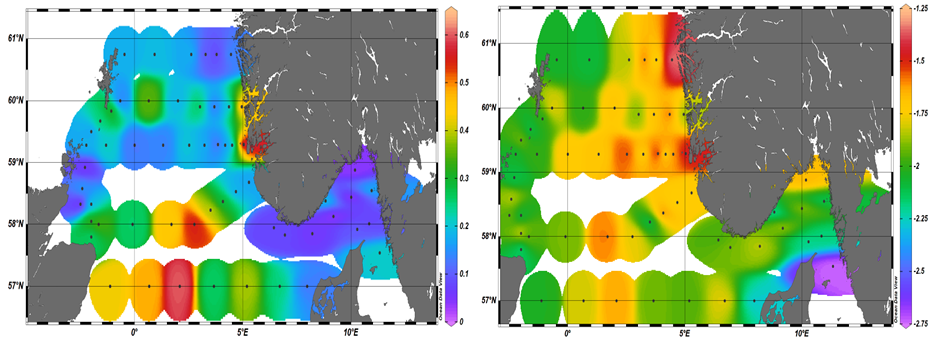
In terms of total zooplankton biomass, we observed high accumulations in the southwest sector of the North Sea (Figure 15 a), where the highest numbers of calanoids copepods were measured. As matter of fact, within the image based Calanoids group, a large percentage of organisms was quite large. Combining these results with microscopy analysis we can suggest that these organisms belonged most likely to Calanus helgolandicus and C. finmarchicus (Figure 20).
Insights on the community size distribution can be extracted from the Flow Cam imaging analysis. For instance, the value of slope derived from the relationship between the number of organisms in each size class and their body volume, gives a measure of the community structure in each sample. Highly negative slope values (colder color) describe communities largely dominated by smaller organisms. While less negative slopes (warmer color) identify communities where the contribution of larger organisms is higher and overall, the community presents a more homogeneous size distribution. Thus, the red colors dominating the Norwegian trench and the northeast sector of the North Sea indicate that the zooplankton community in these areas was characterized by higher percentages of larger organisms (Figure 18b).
Figure 15. Left panel) : Areal distribution of Total zooplankton biomass during the North Sea Ecosystem Cruise 2023002006. Right panel) areal distribution of the slopes derived from the relationship between the number of organisms in each size class and their body volume. Warmer colors indicate a less steep slope and thus a higher contribution of larger organisms to the zooplankton community, while colder colors indicate a larger proportion of smaller organisms.
3.6 - Mesozooplankton
3.6.1 - Zooplankton biomass
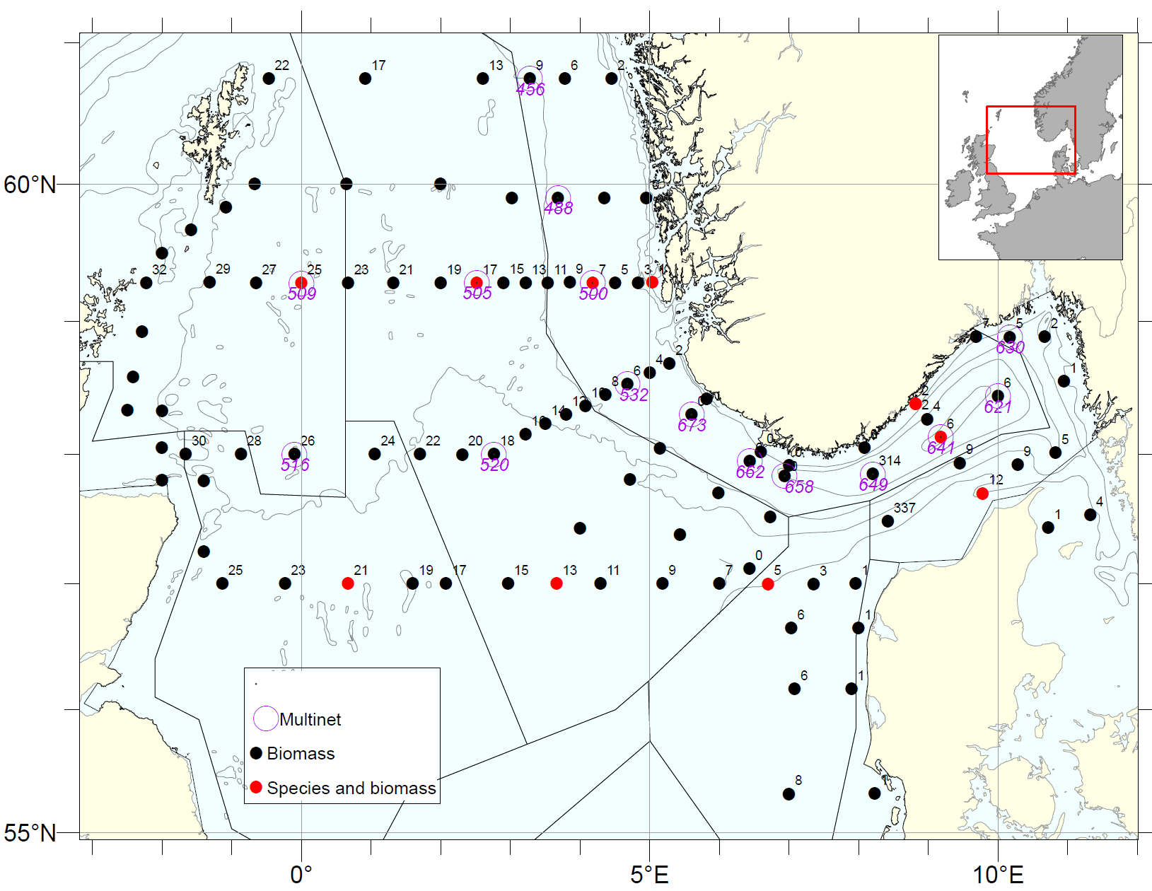
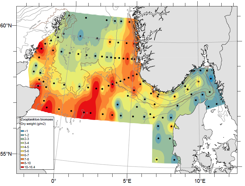
Mesozooplankton sampling during the NSEC 2023 included 105 vertical net tows (WP2), and 15 Multinet hauls (Figure 16). The spatial distribution of total mesozooplankton biomass (dry weight) (Figure 17) is based on the 105 WP2 samples. Overall, the average zooplankton biomass for the whole survey area, was 5.1 g m-2 which is close the long-term average (2005-2022) of 5.7 g m-2. High biomass values were registered at the central and western stations of the Hanstholm-Aberdeen transect (maximum 16.4 g/m2). High biomasses were also recorded along the Norwegian west coast, over the Norwegian Trench (7-8 g/m2). In contrast, lower zooplankton densities (<3 g/m2 ) were recorded in Skagerrak and southeastern part of the survey area (eastern stations on Hanstholm-Aberdeen).
Figure 16. Zooplankton stations on the North Sea Ecosystem cruise 2023. Species compositions were analyzed at selected stations on the transects Utsira-StartPoint, Hanstholm-Aberdeen and Torungen-Hirtshals (indicated with red point.
Figure 17. Distribution of total zooplankton biomass (g dry-weight m-2 ) from near-bottom to surface in the North Sea during the NSEC 2023 (WP2, 180 µm). Interpolation was made in ArcGIS v.10.8.1, module Spatial Analyst, using inverse distance weighting (IDW).
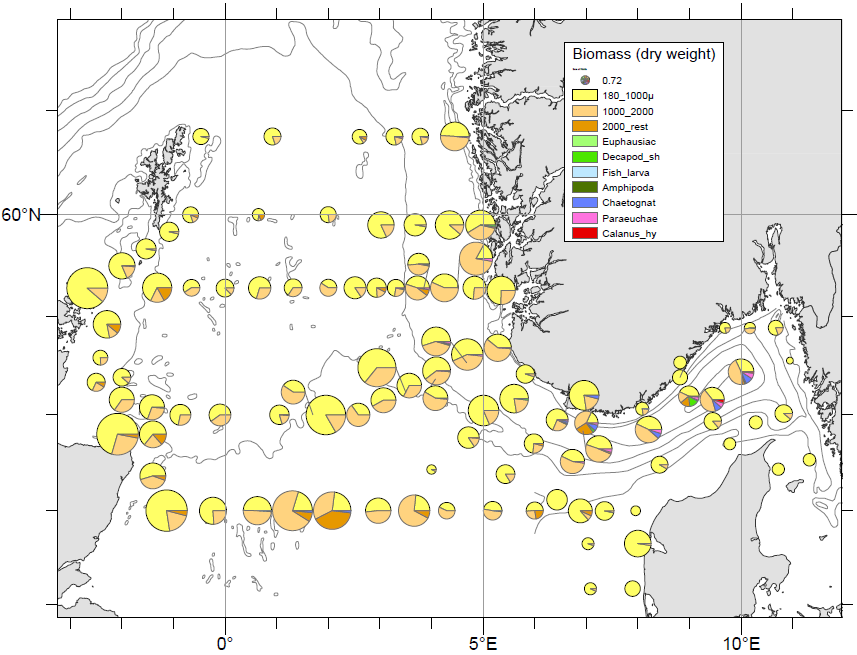
Generally, the zooplankton biomass was dominated by small sized zooplankton (180 -1000 µm), particularly in the western and central part, and made up >60% of the total biomass on most stations (Figure 18). This smallest size fraction contains small sized copepods ( Oithona sp, Pseudocalanus spp), juvenile stages of large copepods ( Calanus spp. ) and benthic larvae. However, this fraction may also contain phytoplankton, which will cause an overestimation of the zooplankton biomass values.
The 1000-2000 µm size fraction, which is dominated by Calanus spp., were more prominent on the Norwegian (eastern) side of the survey area and along the Hanstholm-Aberdeen transect (Figure 18). Larger sized zooplankton (> 2000 µm) including large copepods ( Calanus hyperboreus, Paraeuchaeta norvegica) amphipods, decapod shrimps, and chaetognaths were associated with the deeper stations along the Norwegian trench.
Figure 18 . Relative proportions of zooplankton size fractions in WP2 net tows (180 µm, bottom-surface). Pie chart radii indicating total biomass concentrations.
3.6.2 - Zooplankton taxonomic composition
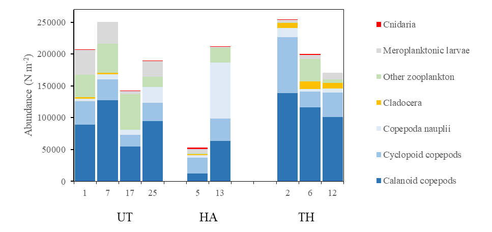
Species identifications and enumeration of zooplankton (WP2 tows) were analyzed at selected stations along the three transects Utsira-StartPoint, Hanstholm-Aberdeen and Torungen-Hirtshals (Figure 19). The North Sea zooplankton community in april 2023 was numerically dominated by copepods. Higher densities of copepods were encountered in Skagerrak (Torungen-Hirtshals transect) and on the Utsira-StartPoint transect, typically dominated by small copepod taxa ( Oithona spp and Para-Pseudocalanus spp). Cladocerans were more numerous in Skagerrak (Torungen-Hirtshals) while meroplanktonic larvae of benthic species were present on the Utsira-transect. Other important groups were larvaceans (Appendicularia), pteropods ( Limacina retroversa ) and euphausiids.
Figure 19. Zooplankton abundance (numbers/m 2 ) on selected stations along three transects Utsira-StartPoint (UT), Hanstholm-Aberdeen (HA) and Torungen-Hirtshals (TH). Positions shown in map, Figure 16.
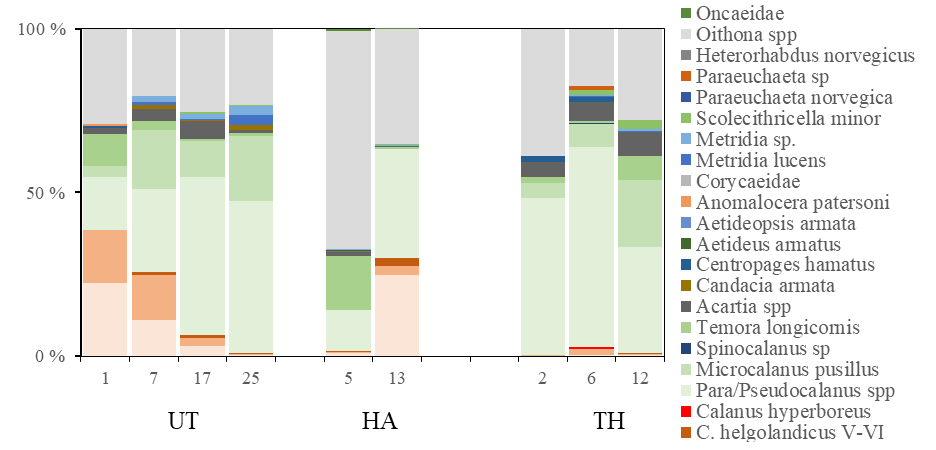
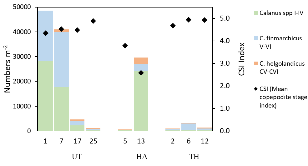
Overall, 44 different taxa (species or genus) of copepods were encountered, and the contribution of different taxa to the copepod community is presented in Figure 20. Para/Pseudocalanus, Calanus spp , Oithona spp, and Microcalanus sp were the most abundant taxa. The deep station in the Norwegian Trench (Torungen-Hirtshals, station 6) comprised a diverse assemblage of arctic-boreal copepod species: Paraeuchaeta norvegica, C. hyperboreus, Aetideopsis armata and Heterorhabdus norvegicus . Calanus spp was most abundant at the northeastern stations (Utsira-StartPoint transect, >40000 ind m -2 , station 1 and 7), while abundances were below 80 ind m -2 in Skagerrak (Torungen-Hirtshals). Both species, C. finmarchicus and C. helgolandicus, co-occurred across the survey area . However, C. finmarchicus was the dominating species on all stations, typically comprising >80% of the Calanus spp CV-CVI (Figure 20 and 21).
Figure 20. Taxonomic composition (%) of copepods on selected stations along three transects Utsira-StartPoint (UT), Hanstholm-Aberdeen (HA) and Torungen-Hirtshals (TH). Positions shown in map, Figure 16.
To explore the stage composition of Calanus , the mean copepodite stage index (CSI) is presented in Figure 6 as an abundance-weighted mean stage (CSI=1 when all CI, and 6 when all adults). The CSI ratio varied between 2.6 and 4.9 which can be interpreted as variations in phenology in different parts of the surveyed area. CSI values less than 3 on the Hanstholm transects, suggests that Calanus was in an earlier phase of the seasonal reproduction in this area compared to stations further north (CSI 4.3-4.9). This may be related to the higher proportion of C. helgolandicus, which have a different phenology (later seasonal reproduction) compared to C. finmarchicus.
Figure 21. Stage composition and species composition of Calanus finmarchicus and C. helgolandicus on selected stations along three transects Utsira-StartPoint (UT), Hanstholm-Aberdeen (HA) and Torungen-Hirtshals (TH). Positions shown in map, Figure 16. Mean copepodite stage index (CSI) is calculated as abundance-weighted average stage number, with ratio ranging between 1 (all CI) and 6 (all adults).
3.7 - Macroplankton
A total of 27 different taxa were recorded in the macroplankton trawl hauls, including fish (11), crustaceans (8) and gelatinous plankton (8 taxa) (Figure 22). The highest densities were registered at the five easternmost stations (0.02-0.01 g/m3, equivalent to 11.3-4.8 g/m2) where bottom depth exceeded 340 m. Considerably lower densities were found in the western and northern part of the trench, where biomass was below 0.01 g/m3 . In the eastern (inner) part of the trench the macroplankton community was dominated by decapods ( Pasiphaea sp) which made up 60-80% of the total biomass. In contrast, euphausiids (mainly Meganycriphanes norvegica) was the dominating taxa at the western and northern stations, with 60-80 % of the total biomass. The gelatinous plankton community also showed clear spatial differences. Aurelia aurita was observed at the northern stations, while Cyanea capillata (and to lesser extent C. lamarckii) was more abundant in the southeastern area. Chaetognaths were also part of the plankton community at the deeper stations in Skagerrak. The Macroplanktontrawl is developed specifically for quantitative sampling of macroplankton and micronekton but is less suited for larger fish species. The fish catches from the macroplankton trawl were generally low, but nevertheless revealed a diverse list of 11 species (Table 6). By weight, the most abundant fish species was Maurolicus muelleri, and Squalus acanthias (eastern stations).
Figure 22. Macroplankton in the Norwegian Trench. a) Stations sampled with the Macroplankton trawl (36 m 2 , 3 mm mesh, oblique hauls bottom-0m); b) Taxonomic composition of macroplankton catches (g wet weight m -3 ); b) Bottom depth along the transect, ranging from 226 to 680 m.
Table 6. Taxa registered in Macroplankton trawl. Densities as wet weight (10-4 g/m3).
Serial number
71033
71032
71034
71035
71037
71043
71042
71041
71040
71039
71038
Station number
456
449
495
500
529
673
662
658
649
302
634
Amphipoda
Amphipoda
0
0
0
0
0
0.41
0
0
0
0
0
Hyperia galba
0
0
0.07
0
0
0
0.19
0.13
0
0
0
Themisto abyssorum
0
0
0.07
0
0
0
1.89
1.29
1.25
2.01
1.94
Decapoda
Caridea
0
0
0.07
0
0
0
0
0
0
0
0
Pasiphaea sp
0
10.94
3.55
0
0
10.52
120.33
77.39
154.07
140.51
71.93
Pasiphaea multidentata
0
0
0
0
0
0
0
0
0
0
5.13
Euphausiacea
Meganyctiphanes norvegica
25.76
42.35
5.83
11.83
41.91
1.39
37.90
7.74
2.50
7.03
5.83
Nematoscelis megalops
0
0
0.40
0
0
0
0
0
0
0
0
Copepoda
Paraeuchaeta cf. norvegica
0
0
0
0
0
2.53
1.89
9.03
3.74
14.05
1.94
Teleostei
Benthosema glaciale
0
0.11
0
0
0
0
0
0
0
0
0
Notoscopelus kroeyeri
0
0
0
0
0
0
0
0
0
0.92
0
Coryphaenoides rupestris
0
0
0
0
0
0.08
0.15
0.07
0.58
0.46
0.39
Maurolicus muelleri
10.28
0.68
0.20
0.85
4.36
1.96
3.12
6.70
0.29
0.05
1.06
Melanogrammus sp
0
0
0
0
0
0
0
0
0.29
0
0
Merlangius sp
0
0
0
0
0
0
0
0
1.59
0
0
Pleuronectiformes
0
0
0.07
0
0
0
0
0
0
0
0
Trisopterus esmarkii
0
0
0
0
0
0
0.59
0.87
0
0
0
Gadidae
0
0
0.07
0.06
0
0
0.37
1.00
0
0.36
0
Teleostei
0
0
0
0
3.19
0.08
0
0
0
0
0
Elasmobranchii
Squalus acanthias
0
0
0
0
0
0
0
6.36
12.11
3.80
0
Chaetognatha
Chaetognatha
0
0
0
0
0
0
2.84
2.58
0
6.02
31.11
Cnidaria
Cyanea sp
0
0
0
0
1.28
0
0
0
0
0
0
Cyanea capillata
0
0
0
0
0
0
7.80
12.05
41.46
16.90
2.61
Cyanea lamarcki
0
0
0
0
0
2.12
1.86
2.68
0.43
0
1.26
Cnidaria
0
0
0
0
0
0
15.67
0
0
0
0
Aurelia aurita
14.72
16.46
0
19.75
1.60
0
0
0
0
0
0
Scyphozoa
0
0
0
0
0
0
0
0
0
0
0.58
Cnidaria indet.
0
0
0
0
0
0
0
0
0.58
0
0
Ctenophora
Pleurobrachia pileus
0
0
0
2.44
0
0.49
0
0
0
0
0
Bottom depth
327
372
226
276
288
332
341
402
523
630
680
Max. Sampling depth
301
347
206
246
259
303
324
384
484
592
655
3.8 - Radioactivity
The Baltic Sea is the largest source of radioactive contamination to Norwegian waters today. The reason for this is that land areas around the Baltic Sea received significant amounts of fallout from the Chernobyl accident in 1986. Run-off from these contaminated land areas is transported with ocean currents from the Baltic Sea to Norwegian waters. To monitor the supply of cesium-137 (Cs-137) to Norwegian waters, we aim to sample seawater from 10 stations in Skagerrak yearly (Table 4, Figure 5).
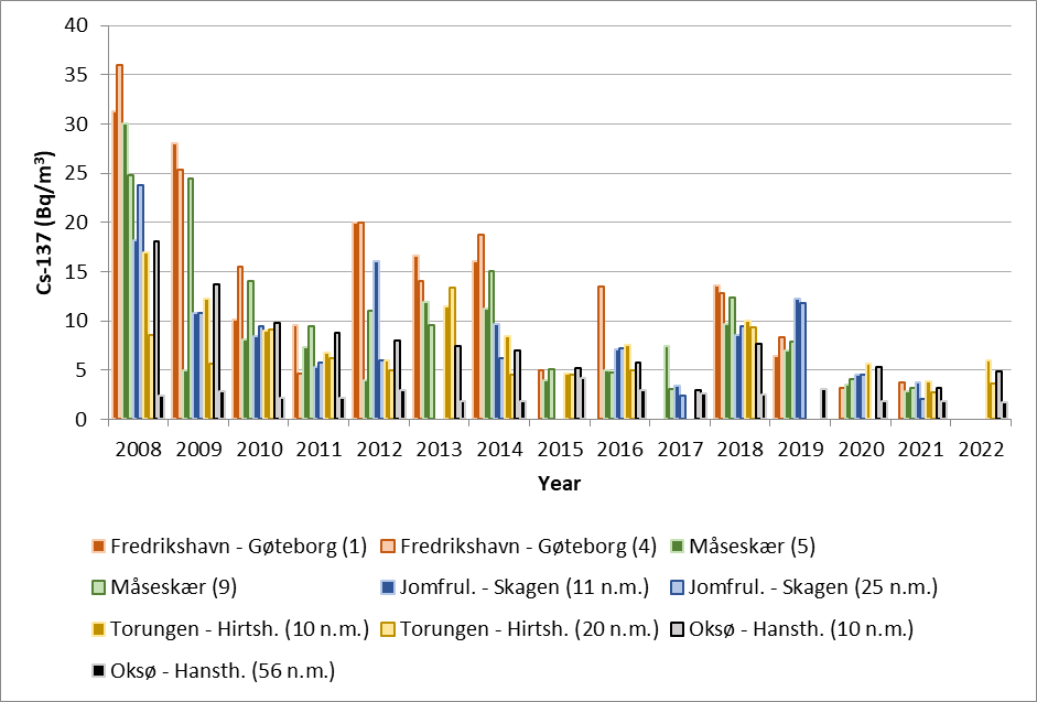
Figure 23. Activity concentrations of cesium-137 (Cs-137) (Bq/m3) in samples of seawater collected yearly in the period 2008 – 2022 at the stations shown in Figure 5.
Results from 2008 to 2022 are shown in Figure 23. In 2022, samples were only collected from the two sections Torungen-Hirtshals and Oksø-Hanstholm. The samples collected in 2023 are not yet analysed. The highest activity concentrations of Cs-137 are, as expected, found at the Fredrikshavn–Gøteborg section, which is nearest the outlet of the Baltic Sea. The lowest activity concentrations are found at the Oksø-Hanstholm section. The activity concentrations of Cs-137 at Oksø-Hanstholm (56 n.m.) have been more or less constant in the period 2008-2022. This is as expected as seawater at this station has characteristics more like the North Sea.
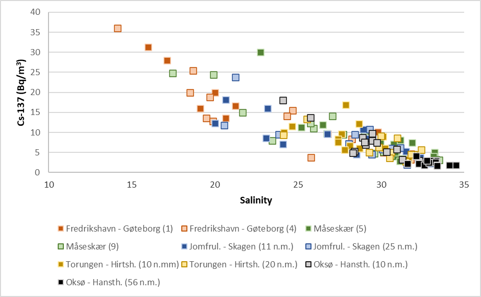
Although there is a constant supply of Cs-137-contamination from land to the Baltic Sea, the data indicate a general decreasing time trend (Figure 23). This is mainly due to radioactive decay of Cs-137, which has a physical half-life of 30 years. Yearly variations in Cs-137 levels are due to variations in precipitation and run-off from land and oceanographic processes, among other things. Figure 24 shows activity concentrations of Cs-137 (Bq/m3 ) at each station plotted against salinity. There is a clear negative correlation between salinity and activity concentrations of Cs-137. The Baltic Sea has brackish water, and the salinity of its surface waters vary from 1–2 in the northernmost Bothnian Bay to around 20 in the Kattegat compared to 35 in the North Sea. Thus, low salinity implies larger degree of “Baltic Sea characteristics”. Higher salinity implies larger degree of “North Sea characteristics”. This generally agrees with our Cs-137-results.
Figure 24. Activity concentrations of cesium-137 (Cs-137) (Bq/m3 ) in samples of seawater collected yearly in the period 2008 – 2022at the stations shown in Figure A plotted against salinity.
3.9 - Metabarcoding
3.9.1 - Sequencing results and overall diversity
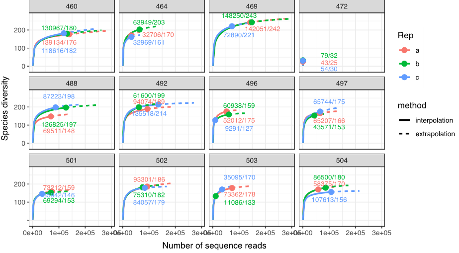
The sequencing run produced 14,010,610 reads, with 52 - 182,000 reads per replicate (mean = 52,671) and 172 - 476,000 reads per sample (mean = 170,861). Rarefaction analysis suggested that ~30,000 reads were sufficient for most samples to recover most of the diversity (slope < 0.001) from the WP2 nets (Figure. 25) and 60,000 reads for the GULF VII nets (not shown). 1 of the 43 WP2 samples and 14 of 39 GULF VII samples failed to produce a sufficient number of reads (<30,000/60,000 reads across 3 replicates).
75% of sequence reads were assigned to either holoplanktonic or meroplanktonic species; 7% belonged to phytoplankton, 5% were non-planktonic organisms, and 12% were unknown. 306 species/taxa of zooplankton (118 species of holoplankton and 188 meroplankton) were recovered within the WP2 samples. The most diverse of these included 48 species of copepods, 42 species of cnidarians, 60 species of polychaetes and 24 species of decapods. Meroplanktonic organisms had the highest diversity and made up the majority of sequence reads (average 60%), with echinoderm larvae being the most abundant group (23% of total reads). Among the holoplankton, copepods were the most abundant group (26% of total reads), of which Pseudocalanus elongatus was dominant.
Figure 25. Examples of 12 rarefaction curves of WP2 samples, with numbers on plot indicating total number of reads/# species recovered per replicate. One sample among the WP2 samples (st. 472), and 14 samples among the GULF VII samples (not shown) failed to produce sufficient reads across all 3 replicates.
Taxa
# of sequence reads
Average % sequence reads
# of species
Most common species
Holoplankton
Calanus spp.
229996
3.2
3
Calanus finmarchicus
Other copepods
1644566
23.2
45
Pseudocalanus elongatus
Amphipoda
516
<0.1
1
Themisto abyssorum
Chaetognatha
123741
1.7
5
Sagitta elegans
Cladocera
8566
0.1
4
Evadne nordmanni
Cnidaria
503664
7.1
42
Nanomia cara
Ctenophora
40145
0.6
2
Bolinopsis infundibulum
Euphausiida
58413
0.8
6
Meganyctiphanes norvegica
Ostracoda
67168
0.9
3
Discoconchoecia elegans
Pteropoda
97103
1.4
5
Limacinidae
Rotifera
1892
<0.1
2
Rotifera
Total
2775770
39.1
118
Meroplankton
Bivalvia
17015
0.2
12
Palliolum tigerinum
Bryozoa
39774
0.6
5
Electra pilosa
Hemic hordata
2222
<0.1
5
Glossobalanus marginatus
Cirripeda
614321
8.7
5
Verruca stroemia
Decapoda
161398
2.3
24
Polybius henslowii
Echinodermata
2570699
36.2
18
Gracilechinus acutus
Fish larvae
154324
2.2
19
Melanogrammus aeglefinus
Gastropoda
161695
2.3
23
Aporrhais pespelecani
Nemertea
91622
1.3
16
Tubulanidae
Polychaeta
482336
6.8
60
Paramphinome jeffreysii
Phoronida
26795
0.4
1
Phoronis muelleri
Total
4322201
60.9
188
Table 7. Summary of taxonomic diversity recovered via metabarcoding (WP2 net data only).
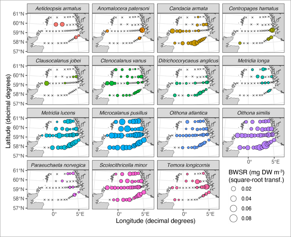
Species distributions based on BWSR
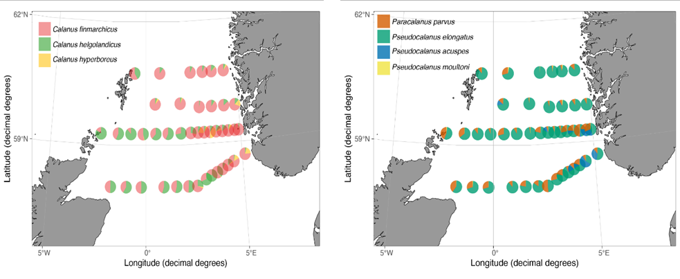
Species-specific BWSR (% sequence reads multiplied by total zooplankton biomass) revealed distinct patterns in zooplankton distribution (Figure 26--28). For example, the northern and eastern region of the North Sea was characterized by the dominance of Calanus finmarchicus and the presence of C. hyperboreus , while the western and southern region was dominated by C. helgolandicus.
Figure 26. BWSR distribution of the most common copepod species (WP2 net only), excluding Calanus spp. and Pseudo/Paracalanus spp.
Figure 27. BWSR distribution of the most common fish species (GULF VII net only).
Figure 28. Left panel: Relative composition of Calanus spp.; Right pane:) Relative composition of Pseudo-/Paracalanus spp (WP2 net only).
The described protocol is a promising addition to zooplankton monitoring programs, recovering a much higher diversity than is possible with microscopic analysis and revealing distinct patterns in zooplankton distribution. However, the low sequencing success of some samples (particularly from the GULF VII net), as well as the low contributions of some groups compared to their expected presence in the sample (i.e. Calanus spp.) suggests that some DNA degradation took place, likely during the freeze-thaw cycles, which possibly favored some taxonomic groups over others. To improve DNA quality, it is recommended to (a) flash freeze the samples in liquid N, (b) add buffer to stabilize DNA and reduce enzyme activity, (c) lyophilize the frozen samples prior to extraction. A new set of experiments testing these modifications, as well as comparing the efficacy of this method of preservation compared to traditional ethanol preservation, will take place in spring 2024.
3.10 - Ichthyoplankton
A total of 89 GULF VII hauls were conducted during the survey. Results presented here are preliminary, as fish larvae and eggs could only be identified to higher taxonomic groups while at sea, due to time constraints, with identification to species level and quality assurance pending.
3.10.1 - Fish eggs
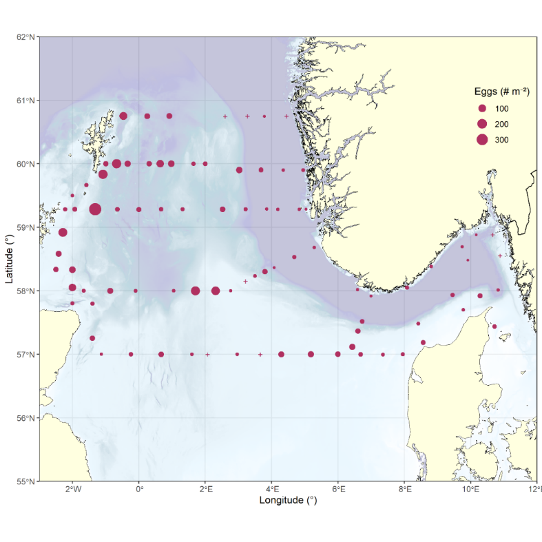
Fish eggs were found at almost all stations, with highest densities per m 2 (384 eggs m -2 ) observed southeast of Fair Isle with the area east and southeast of Shetland exhibiting an overall center of abundance, and a consistent decline east- and southwards with lowest densities observed over the Norwegian trench (Figure 29). Notable is a local peak in abundance east of the Devil’s hole, breaking the general trend of decrease towards the Southeast.
Figure 29. Distribution of fish eggs during the survey, raised to numbers per square meter (# m -2 ).
3.10.2 - Fish larvae
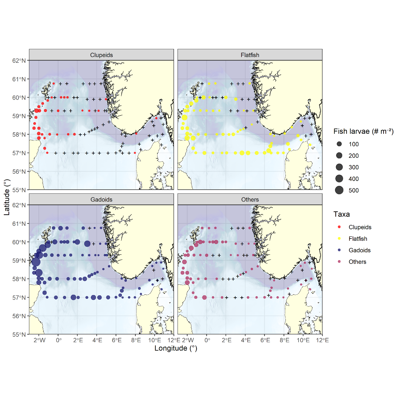
Like with fish eggs, the highest densities of fish larvae were observed on the western edge of the survey area (Figures 30, 31a), dominated by Gadoids with a peak density of 600 m -2 east of Orkney. Clupeids were found almost exclusively along the Fair Isle - Pentland transect, but much lower in abundance, peaking at 59 m -2 . Flatfish comprise the taxonomic groups of Pleuronectidae and Scophtalmidae . Whilst also peaking east of Orkney (159 m -2 ) and being predominately found on the western edge of the survey area, flatfish exhibited an overall more southerly distribution. Stations without flatfish were common in the eastern parts of the northern transects, whilst nearly all stations on the Jaeren’s Rev transect and all stations on the Hanstholm - Aberdeen transect contained flatfish. In the latter transect a secondary cluster of abundance was found on the eastern part of the Little fisher bank (Figure 30). Similar to Clupeids the diverse group of other species, containing among other argentines, gobies and dragonets, was most commonly found in the western part of the North Sea, peaking at 92 m -2 . Unlike Clupeids this group was also prominent in the Southeast and the Skagerrak. Generally, diversity was greater at stations at the western and eastern margins of the survey area, where it bounded with other seas.
Figure 30. Distribution of larvae separated by large taxonomic or functional groups. Gadoids dominated the assemblage, being found almost everywhere and exhibiting the highest densities, with Clupeids representing the other extreme of the range, being nearly exclusive to the western part of the survey area and having peak densities a tenth of the Gadoids. The group Others comprises a wide range of species, including argentines, gobies and dragonets.
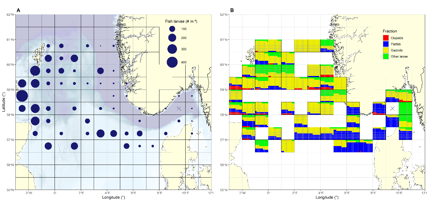
Aggregating the assemblage to ICES rectangles, it can be shown that the assemblage north of 58°N was dominated by Gadoids, making up 100% of the species composition in several rectangles along the Feie - Shetland and Utsira - Startpoint transects (Figure 31 right panel). Further south, the larval assemblage was still dominated by Gadoids west of 2°E with flatfish gradually increasing towards the East and dominating the larval community in the rectangles corresponding to the Fisher and Jutland banks and into the Skagerrak. Rectangles east of 10°E and southeast of Shetland exhibited a high proportion of other species, potentially because of the mingling with assemblages from adjacent seas.
Figure 31. Left panel) Total abundance of fish larvae and right panel) proportional composition of the larval assemblage aggregated by ICES rectangles. Gadoids dominated the assemblage and the abundance north of 58°N and in the southwestern part of the survey area. There was a gradual increase of flatfish from west to east, with their proportion in the assemblage peaking around the Fisher banks and the Skagerrak.
3.10.3 - Relationships to the abiotic environment
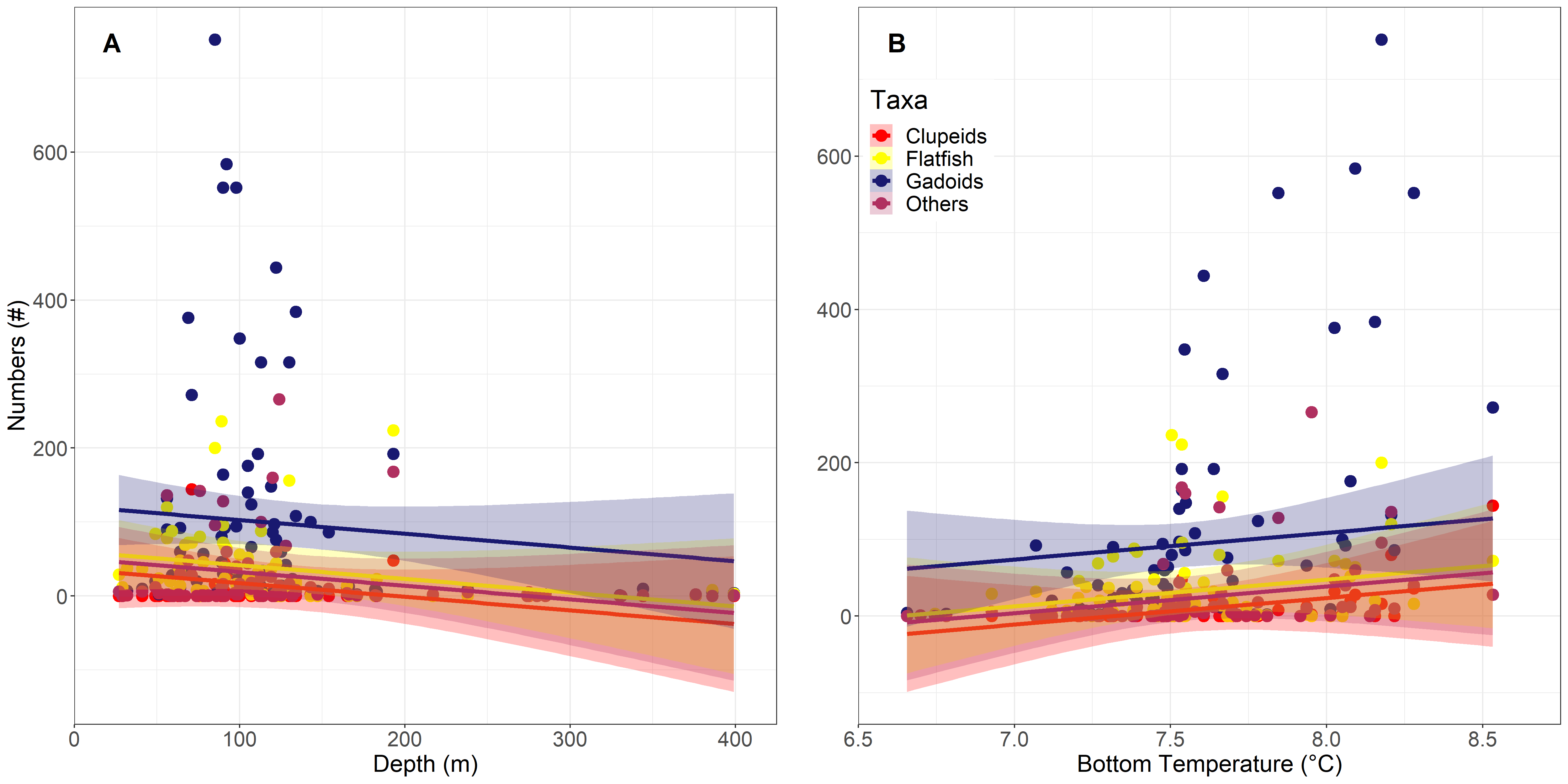
The GLMM using near-bottom temperature exhibited a slightly lower AIC of 4622.1 than the model using the surface layer temperature. Additionally, temperature as well as depth were both highly significant in this model (p<0.001), whilst temperature in the surface model was of lesser significance (p=0.02). In both models Gadoids were significantly different from other groups. However, all taxa exhibited the same negative relationship to depth and positive relationship to temperature, with declining and increasing trends, respectively.
Figure 32. GLMM for the relationship between A) larval abundance and depth and B) the relationship to near-bottom temperature. Trends are towards higher abundances at shallower depth, peaking at around 100 m depth and higher temperatures, with peak abundances between 7.5°C and 8.75°C. Whilst the trends were the same for all groups, the slope varied noticeably for flatfish and Gadoids were significantly different to other groups.
4 - Acknoledgments
We greatly appreciate and thank the masters and crew onboard RV Johan Hjort for the collaboration and practical assistance during the North Sea Ecosystem cruise 2023. We would like also to express our sincerest gratitude to all technicians of the plankton group who provided invaluable contributions, both during the collection and processing of samples onboard, as well as the meticulous analyses conducted in the laboratories. Your expertise, dedication, and tireless efforts have been instrumental in the success of this endeavor and essential in producing reliable data. A special thank you for this year work goes to: Gaston Ezequiel Aguirre, Terje Berge, Eli Gustad, Mona Ring Kleiven, Linda Fonnes Lunde, Hege Lyngvær Mathisen, Jane Strømstad Møgster, Magnus Reeve, Jon Rønning, Hege Skaar and Hilde Arnesen Øyjordsbakken.
5 - References
Brooks, M. E., K. Kristensen, K. J. van Benthem, A. Magnusson, C. W. Berg, A. Nielsen, H. J. Skaug, M. Maechler, and B. M. Bolker. 2017. “glmmTMB Balances Speed and Flexibility Among Packages for Zero-Inflated Generalized Linear Mixed Modeling.” The R Journal 9 (2): 378–400. https://doi.org/10.32614/RJ-2017-066.
Ershova E.A., Wangensteen O.S., Descoteaux R., Barth-Jensen C., Præbel K. (2021) Metabarcoding as a quantitative tool for estimating biodiversity and relative biomass of marine zooplankton. ICES Journal of Marine Science, 78(9) 3342–3355, https://doi.org/10.1093/icesjms/fsab171
GEBCO Compilation Group. 2023. “GEBCO 2023 Grid.”
Heino, M., Porteiro, F.M., Sutton, T.T., Falkenhaug, T., Godø, O.R., Piatkowski, U., 2011. Catchability of pelagic trawls for sampling deep-living nekton in the mid-North Atlantic. ICES Journal of Marine Science 68, 377–389.
Hiemstra, P. H., E. J. Pebesma, C. J. W. Twenhöfel, and G. B. M. Heuvelink. 2008. “Real-Time Automatic Interpolation of Ambient Gamma Dose Rates from the Dutch Radioactivity Monitoring Network.” Computers & Geosciences.
Nash, R. D. M., M. Dickey-Collas, and S. P. Milligan. 1998. “Descriptions of the Gulf VII/PRO-NET and MAFF/Guildline Unencased High-Speed Plankton Samplers.” Journal Article. Journal of Plankton Research 20: 1915–26.
R Core Team. 2023. R: A Language and Environment for Statistical Computing. Vienna, Austria: R Foundation for Statistical Computing. https://www.R-project.org/.
Roos P., 1994. Comparison of AMP precipitate method and impregnated Cu2[Fe(CN)6] filters for the determination of radiocesium concentrations in natural water. Nuclear Instruments and Methods in Physics Research Section A: Accelerators, Spectrometers, Detectors and Associated Equipment. Volume 339, Issues 1–2, 22 January 1994, Pages 282-286
Skjerdal, H., Heldal, H.E., Gwynn, J., Strålberg, E., Møller, B., Liebig, P.L., Sværen, I., Rand, A., Gäfvert, T., Haanes, H. (2017). Radioactivity in the Marine Environment 2012, 2013 and 2014. Results from the Norwegian National Monitoring Programme (RAME). StrålevernRapport 2017:13. Østerås: Norwegian Radiation Protection Authority.
Skjerdal, H., Heldal, H.E., Rand, A., Gwynn, J., Jensen, L.K., Volynkin, A., Haanes, H., Møller, B., Liebig, P.L., Gäfvert, T. (2020). Radioactivity in the Marine Environment 2015, 2016 and 2017. Results from the Norwegian Marine Monitoring Programme (RAME). DSA Report 2020:04. Østerås: Norwegian Radiation and Nuclear Safety Authority.
Utermöhl, H. 1958. Zur Ver vollkommung der quantitativen phytoplankton-methodik. Mitteilung Internationale Vereinigung Fuer Theoretische unde Amgewandte Limnologie 9: 39.
Wangensteen O.S., Palacín C., Guardiola M., Turon X (2018) DNA metabarcoding of littoral hard-bottom communities: high diversity and database gaps revealed by two molecular markers. PeerJ 6:e4705 https://doi.org/10.7717/peerj.4705
Wenneck, TdL., Falkenhaug T., Bergstad OA (2008). Strategies, methods, and technologies adopted on the R.V. G.O. Sars MAR-ECO expedition to the Mid-Atlantic Ridge in 2004. Deep Sea Research II. 55: 6-28.