Effekter av seismisk støy på dyreplankton (ZoopSeis) er et prosjekt finansiert av Norges Forskningsråd, som har som mål å avdekke effekten av seismikk på dyreplankton. Dette felt eksperimentet, hvor vi tester effekten av seismisk på dødelighet og atferd hos dyreplankton under reelle forhold på Ekofisk, ble muliggjort av et samarbeid mellom ZoopSeis-prosjektet og Glider II prosjektet som ledes av Aquaplan-niva og finansieres av ConocoPhillips. Studeit ble gjennomført med forskningsfartøyet RV Kristine Bonnevie i perioden 29 april til 8 mai 2022. Under undersøkelsen gjennomførte vi tre separate replikate eksperiment. Eksperimentene bestod i at forskningsfartøyet plasserte seg ved enden av en seismisk skytelinje. Fra enden av skytelinjen tok vi dyreplankton prøver mens seismikkfartøyet skjøt seismikk langs skytelinjen opp mot oss og til det passerte forskningsfartøyet. Dette for å få et mål på hvordan avstanden til seismikk skipet / luft kanonen påvirker dødelighet og atferd til dyreplanktonet. Videre brukte vi autonome USV-er (Otter og en kajakk) med akustisk, som fulgte det eksponerte dyreplanktonet mens det drev av fra den faste posisjonen ved enden av skytelinjen. I tillegg ble det brukt bunn fortøyd ekkolodd (WBAT), de ble plassert i enden av de tre skytelinjene før den seismiske undersøkelsen startet. Det ble ikke skutt seismikk i en omkrets på ca 2 km fra det eksperimentelle skytelinjen de siste 48 timene før forsøkene startet. Det ble tatt dyreplankton prøver over hele vannsøylen (~70 m) ved hjelp av WP2 plankton håv. Den største avstanden mellom prøvetakingsnettet og luftkanonene var ~16 km ved starten av linjen, og avstanden ved passasje varierte mellom 46-116 m for de tre eksperimentelle kjøringene. Vi farget planktonprøvene med Red Staining for å synligjøre mengde levende og dødt dyreplankton. Fargede prøver ble delt i tre deler en for fotografering, en ble frosset og en ble konservert i formalin. I tillegg til nettprøvetaking og akustiske data, satte vi ut poser med kultiverte hoppekreps Calanus finmarchicus eller viltfanget hoppekreps. Dette ble gjort både ved starten av de tre seismikk skytelinjene, når seismikkfartøyet var langt unna, og i det øyeblikket seismikkfartøyet passerte oss. Disse hoppekrepsene ble fulgt individuelt over tid for å studere forsinket dødelighet etter eksponering. Samtidig ble det satt ut bur laget av plankton-nett med 3D kamera. I disse filmet vi hoppekrepsens adferd når den ble eksponert for seismikk. Lyden fra den seismiske undersøkelsen ble registrert med omnidireksjonelle hydrofoner. En hydrofon hang under forskningsskipet og registrere lyd på 10 m dyp under de tre eksperimentelle kjøringene. En annen hydrofongruppe registrert lyd på 8 og 35 m dybde i en 24-timers periode hvor det både ble - og ikke ble skutt seismikk. Et døgn under toktet var bølgehøyden for høy til at en kunne skyte seismikk. Dette døgnet ble brukt til å kjøre kontroll eksperiment. I tillegg til in-situ prøvetakingen gjort på toktet, vil Glider II prosjektet til Akvaplan-niva, med sin seilbøye Echo 333Khz bidra med akustisk data fra før under og etter den seismiske aktiviteten. Videre vil Glider II prosjektet bidra med lyd data fra en bunnsatt lander med hydrofon (ett år) og en glider Slocum G3 (vannsøyle CT-profil og JASCO Observer-hydrofon). Sistnevnte satte vi ut i begynnelsen av toktet. Resultatene fra toktet vil bli publisert i fagfellevurderingsartikler når de innsamlede data er ferdig analysert.
Does seismic have an effect on zooplankton?
— Field study at Ekofisk with RV Kristine Bonnevie
Rapportserie:
Toktrapport 2022-9
ISSN: 1503-6294
Publisert: 18.08.2022
Oppdatert: 16.09.2024
Toktnr: 2022611
Prosjektnr: 15653
Oppdragsgiver(e): Norges Forskningsråd
Referanse: Prosjektnummer: 302675
Forskningsgruppe(r):
Økosystemakustikk
,
Plankton
,
Fangst
Tema:
Plankton,
Seismikkprosjekter,
Tobis
Program:
Nordsjøen
Research group leader(s):
Rolf Korneliussen (Økosystemakustikk)
Approved by:
Research Director(s):
Geir Huse
Program leader(s):
Henning Wehde
English summary
Sammendrag
Effects of seismic sound on zooplankton (ZoopSeis) is a project funded by the Norwegian Research Council, aiming at uncovering the effect of seismic on zooplankton. An experiment to test the effect of a real seismic survey on mortality and behaviour at Ekofisk was made possible by a collaboration between the ZoopSeis project and the Glider II project which is led by Akvaplan-niva and funded by ConocoPhillips. The study was conducted with the research vessel RV Kristine Bonnevie in the period 29 April to 8 May 2022. During the survey we conducted three separate experimental runs. During the experimental runs the research vessel sampled zooplankton at a fixed location at the end of a shooting line while the seismic vessel shot seismic along the shooting line until it passed the research vessel. Further, we used autonomous USV’s (Otter and a kayak) holding acoustic transducers, to follow the exposed zooplankton as it drifted off from the fixed position at the end of the shooting line. In addition, landers with upward looking echosounders (WBAT’s) were moored at the end of the three shooting lines before the seismic survey started. Wild zooplankton was sampled with a WP2 net over the entire depth range (~70 m). The largest distance between the sampling net and the airguns was ~16 km at the start of the line, and the distance at passage varied between 46-116 m for the three runs. There was a 48 hour “before” period before each run, in which no seismic was shot within 2 km of the experimental transect. Plankton samples were stained to assess mortality. Stained samples were split into three parts one for photographing, one was frozen, and one was preserved in formalin. In addition to net sampling and acoustic data, we deployed bags with either cultured Calanus finmarchicus or wild-caught zooplankton, both at the start of the transect when the seismic vessel was far away, and at the moment the seismic vessel passed. These plankton were followed individually over time to study delayed mortality after exposure. At the same time, a cage was deployed to document zooplankton behaviour during exposure on video. The sound of the seismic survey was recorded with omnidirectional hydrophones. One hydrophone recorded at 10 m depth at the sampling locations during sampling, and a hydrophone array recorded at 8 and 35 m depth for a 24-hour period at a single location. One day during the cruise the wave height was too high to shoot seismic, this day was used to take control samples and run experimental controls for the bag and cage experiment. In addition to the in-situ sampling done on the cruise, will the Glider II project by Akvaplan-niva provide acoustic baseline data from before during and after the seismic activity with their Sail-buoy Echo 333Khz. Further, will the Glider II project provide data from a lander with hydrophone (one year) and a glider Slocum G3 (water column CT profile and JASCO Observer hydrophone), the later was deployed at the beginning of the cruise. The results and findings from this field study will be published in separate peer review papers after further scrutinizing of the collected data.
1 - Introduction
This report is from a cruise (cruise nr. 2022611) with RV Kristine Bonnevie to Ekofisk North sea 29th of April to 8 th of May 2022 were we looked at the affect of seismic on zooplankton short and long term survival and behaviour. This study was a collaboration with Akvaplan-niva and ConocoPhillips.
The Institute of Marine Research (IMR) is responsible for giving scientific advice on the seismic activity in Norway, with the objective to prevent negative effects on marine ecosystems. Current practice does not consider the effects of seismic blasts on zooplankton, as any potential effects have been assumed to be highly localized, based on studies of fish larvae (Booman et al. 1996). However, a study from Australian waters, McCauley et al. (2017), reported zooplankton mortality up to 1200 m from a seismic transect and infer a causal relationship. The peak abundance of copepods coincides with the period of highest seismic activity. If similar mortality occurs in Norwegian waters, the impact of seismic explorations could have serious consequences for the food web, and thereby for the fisheries, in these highly productive areas.
On the other hand, a recent study performed in Norwegian waters (Fields et al. 2019), found 9 % higher instantaneous mortality at distances closer than 5 m from the source and no effect on escape performance at any distance from the seismic blast. The effects of seismic airgun blasts on Calanus finmarchicus reported by Fields et al. (2019) are much less than reported by McCauley et al. (2017) and those used in models to assess the broader impacts of seismic surveys on zooplankton (such as Richardson et al., 2018). However, the airgun used in Fields et al. (2017) was a small airgun and not a real airgun arry, like we tested in our Ekofisk filed study.
1.1 - OBJECTIVES AND GOALS OF THE SURVEY
Effects of seismic sound on zooplankton (ZoopSeis) is a project funded by the Norwegian Research Council, aiming at uncovering the effect of seismic on zooplankton. This cruise is part of the ZoopSeis project. The aim of the cruise was to find at what distance a full-scale seismic array impacts zooplankton in terms of immediate mortality, delayed mortality and behaviour (e.g. swarming and avoidance).
In addition to this experiment on the zooplankton response to a seismic survey we conducted an acoustic transect on Vikingbanken on our way back. The transect lasted 10 hour covering ~93 nm. The methods followed standard acoustic survey coverage. The acoustic data was scrutinised following the IMR standard sandeel protocol.
1.2 - CRUISE PARTICIPANTS
| Name | Institute | Country | Status |
|---|---|---|---|
| Josefin Titelman | University of Oslo | Sweden | Researcher |
| Thor Klevjer | Institute of Marine Research | Norway | Researcher |
| Geir Pedersen | Institute of Marine Research | Norway | Researcher |
| Espen Strand | Institute of Marine Research | Norway | Researcher |
| Karen de Jong | Institute of Marine Research | Norway | Researcher |
| Atle Totland | Institute of Marine Research | Norway | Technician |
| Sigurd Hannaas | Institute of Marine Research | Norway | Technician |
| Marina Mihaljevic | Institute of Marine Research | Norway | Technician |
| Rune Strømme | Institute of Marine Research | Norway | Technician |
| Reidar Johannesen | Institute of Marine Research | Norway | Technician |
| Håvard Johnsen Buschmann | Akvaplan-niva | Norway | Technician |
| Saskia Kühn | Kiel University | Germany | PhD student |
| Emilie Hernes Vereide | University of Oslo / IMR | Norway | PhD student |
| Anne Christine Utne Palm | Institute of Marine Research | Norway | Researcher, Cruise leader |
2 - Methods and Results
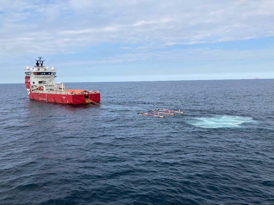
The experimental approach consisted of acoustic monitoring and net sampling during the approach of a seismic vessel, Skandi Nova. Three landers (WBATs) were deployed at Ekofisk by a suply ship of ConocoPhillips prior to the survey (April 12th). Each one of them at the end of separate seismic shooting lines. The three WBATs were holding upward looking echosounders (see section 2.1.1). During the survey three replicate experiments were performed by positioning the IMR research vessel RV Kristine Bonnevie close to each of these three WBATs, while the seismic vessel was approaching us along the shooting line at a speed of 4.5 knots (Figure 1).
The sampling during an approach allowed for the documentation of effects of seismic at different distances (~16 km to ~50 m). Plankton net samples (WP2) were taken continuously as the seismic vessel approached RV Kristine Bonnevie, and with increasing sampling frequently as the seismic vessel got closer.
The set-up used in McCauley et al. (2017) did not allow for testing whether zooplankton mortality could have been caused by other sources of disturbance, such as the propeller wake of the ships used in the experiment or variation in natural mortality over the day (Bickel et al. 2011; Tang et al. 2019). We therefore used autonomous USV’s (Otter and a kayak) holding acoustic transducers, to follow the potentially affected plankton. As an additional control for the effect of propeller we placed zooplankton in plastic bags and lowered them to 10 m for 15 sec. This plastic bag exposure was also done in an increasing frequency as the seismic vessel was getting closer.
Furthermore, we looked at effect of seismic on zooplankton behaviour. This was done by placing zooplankton in a plankton net cage holding a 3D camera set-up (see Fig. 11). Zooplankton behaviour was filmed as the seismic vessel approached and during no shooting period as a control.
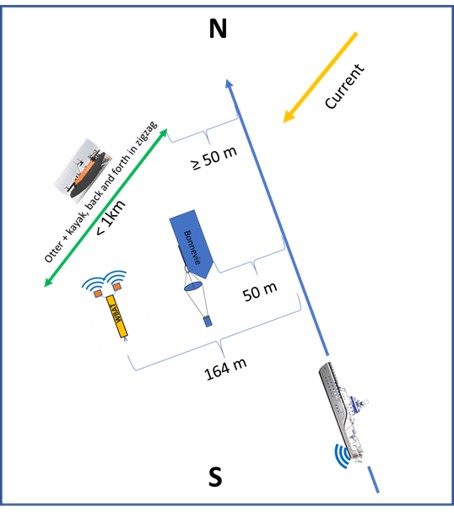
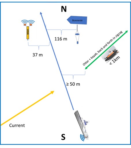
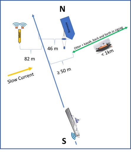
Current was predicted using the North West Shelf model and comparing these with ADCP measurements of the vessel. The two autonomous USV’s (Otter and kayak) was following exposed zooplankton down current as it was drifting off from the seismic shooting line. This was done to look for any sinking or changes in the acoustic plankton layers after seismic exposure – an behavioural phenomenon observed in the acoustic data of McCauley et al. (2017).
2.1 - MULTIFREQUENCY ACOUSTIC SAMPLING AND ANALYSIS
(Geir Pedersen, IMR )
Three main experiments were performed at the site of three pre deployed landers (WBAT 1, 2 and 3) (see section 2.1.1.). In addition to experiments and sampling of copepods, acoustic measurements were performed by multiple platforms.
In addition to the three WBATs RV Kristine Bonnevie collected acoustic data from a fixed position, while two autonomous USV’s vessels (Otter and kayak) performed 500 m transect in parallel with the current direction (see section 2.1.2.) at the three WBAT stations (see Fig. 1). Furthemore, acoustic baseline data from before during and after the seismic activity was collected by Akvaplan-niva's Sail-buoy Eco 2 equiped with an EK80 (333kHz) in adition to CTD and oxygen sensor. The Sail-Buoy run transects in the northern part of the seismic area, near our three WBAT stations.
2.1.1 - The WBAT’s
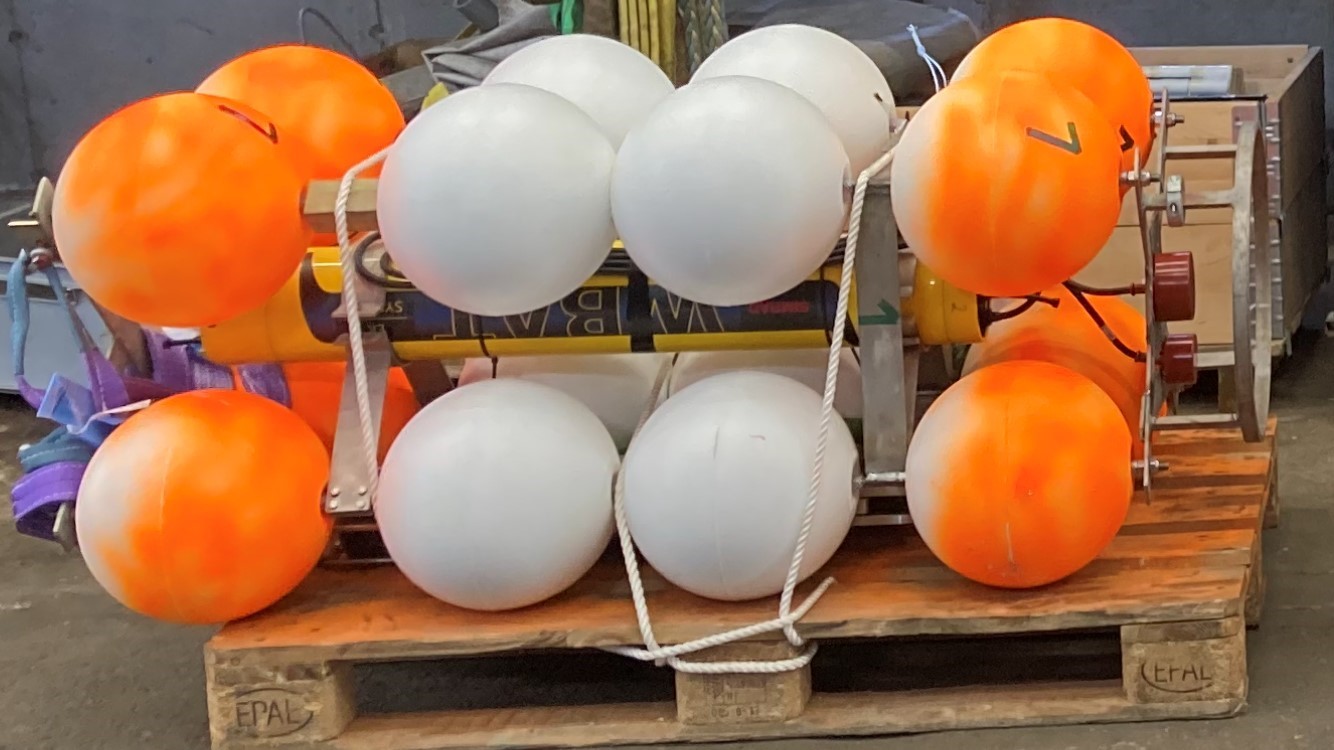
WBAT is based on the same technology as the Wide Band Transceiver (WBT), however as with the Simrad EK80, the WBAT is capable of split-beam operation, which means that it can be calibrated to the same standards and with the same methods as the Simrad EK80. The WBATs continuously collected data from a fixed position from 5 m above the seafloor. We located the position of the 3 WBATs using the acoustics of Kristine Bonnevie (Table 1, and Fig 2). The three WBAT’s holds EK80’s for details see Table 1. The weight of the three landers were ~200 kg (Fig. 3).
| Latitude | Longitude | Transceiver | |
|---|---|---|---|
| WBAT 1: | 56° 34,952 min | 003° 8,269 min | 70 and 200 kHz |
| WBAT 2: | 56° 36,416 min | 003° 13,362 min | 200 kHz |
| WBAT 3: | 56° 36,124 min | 003° 15,476 min | 200 and 333 kHz |
We were not able to retrieve WBAT 1 and 3 at the end of the cruise due to issues with the acoustic release. ConocoPhillips retrieved the last two WBATs by the use of ROV on the 11th of May.
2.1.2 - The USV’s
The two autonomous vehicles were also equipped with Simrad EK80 echosounders. The Kayak hold an ES200-7CD, and the Otter a ES38/200, 333CD. Both vehicles employ electric propulsion.
Otter
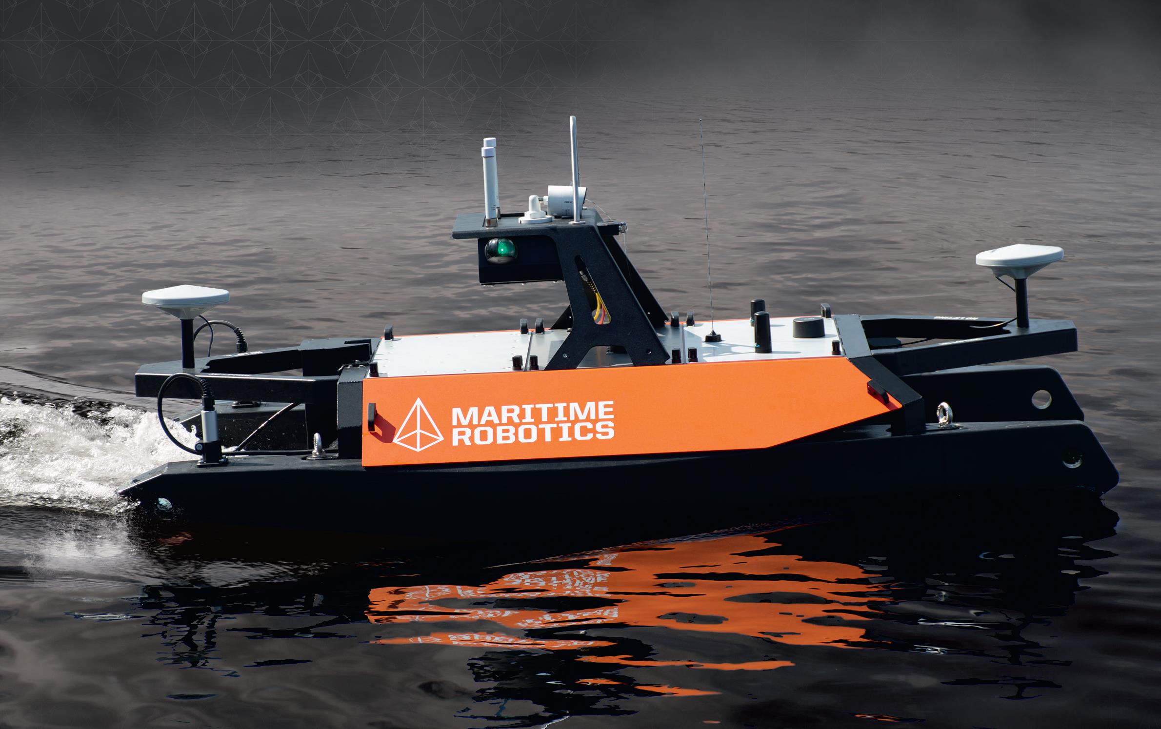
The Otter, owned by Akvaplan-niva, is the smallest member of the Maritime Robotics USV family. Dimensions 200 x 108 x 106.5 cm and weight of 65kg. Akvaplan-niva's Otter holds a EK80 (200 - 38 kHz and 333 kHz transducers). The ES38 and 333 are installed on a pole just below the waterline. For more details see https://www.maritimerobotics.com/otter and Fig. 4
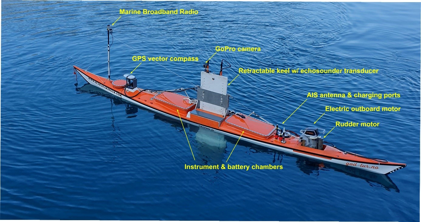
Kayak
The kayak is build by IMR. It is 700 cm long and weighs 300 kg. It holds an EK80 200 kHz transducer. For more details see Fig. 4. The ES200 is installed on a protruding keel (~0.5 m bellow water).
2.1.3 - Seismic experiment
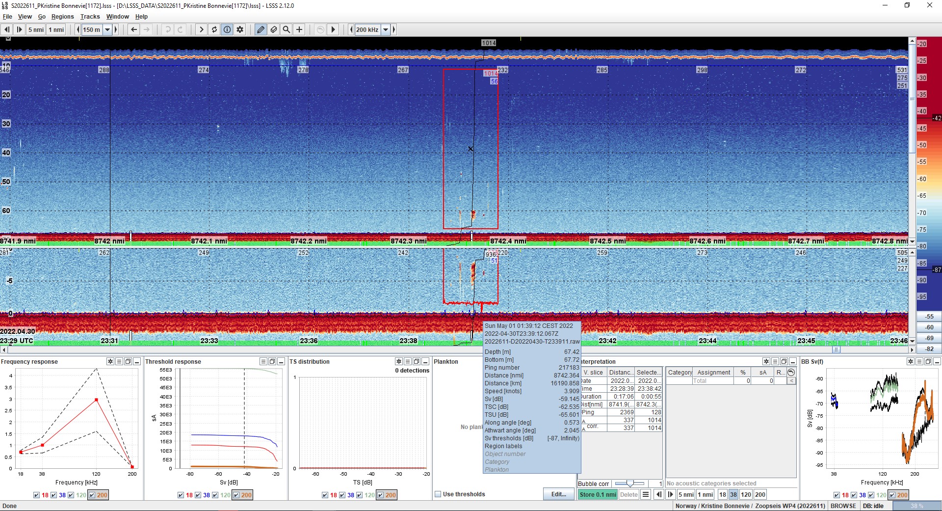
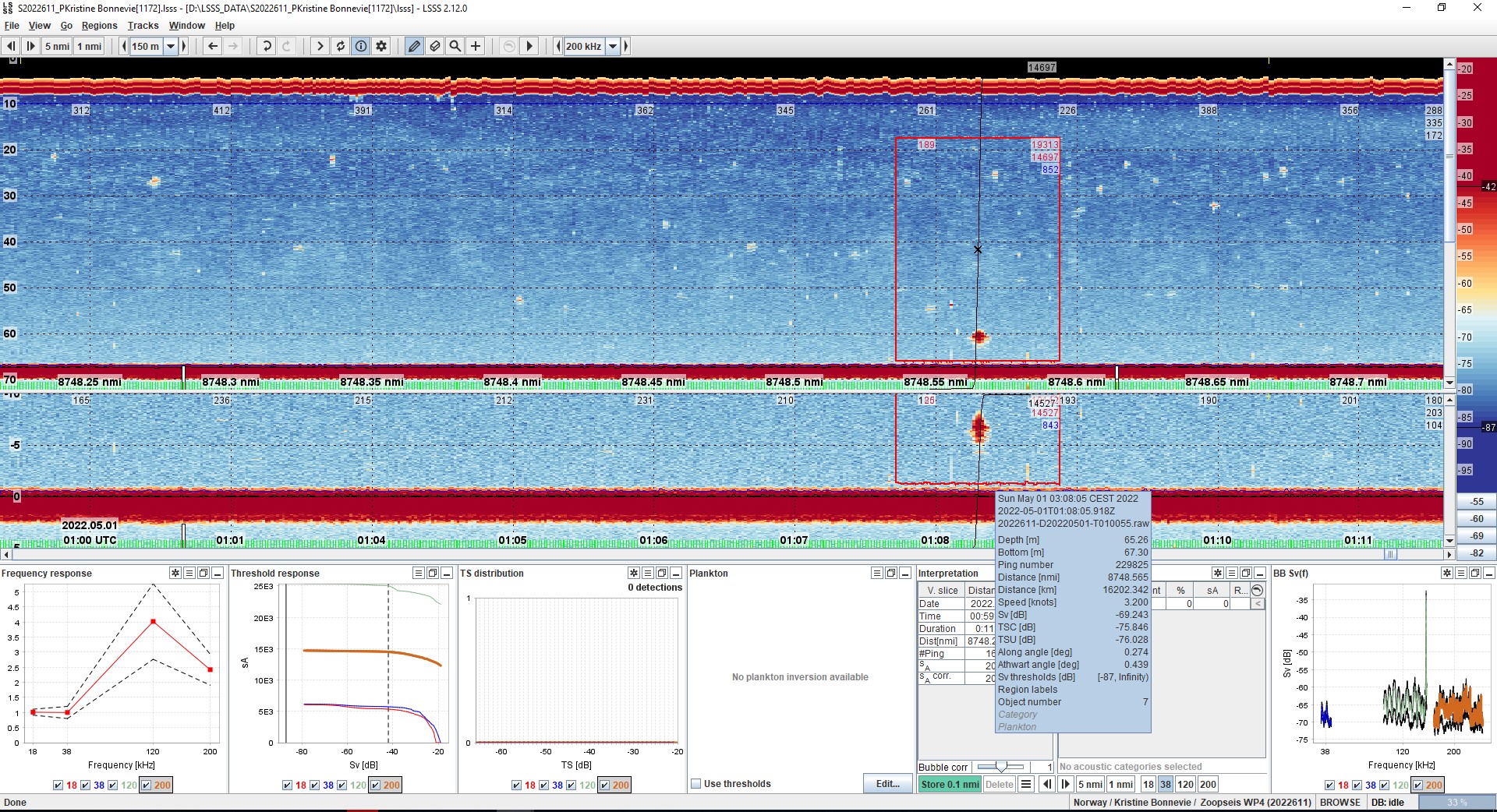
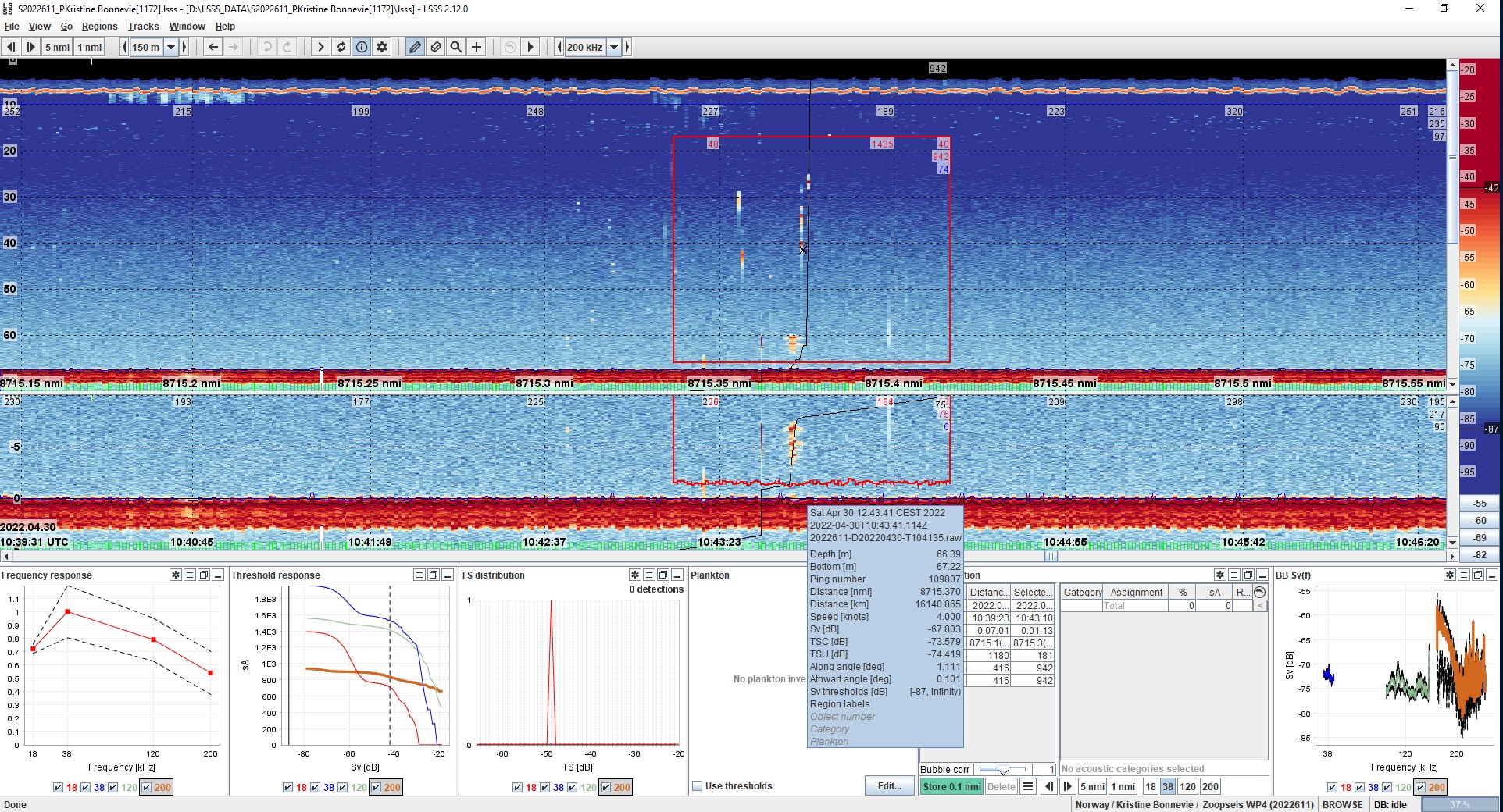
For the seismic experiments (WBAT1-3) each transect was isolated and acoustic data from each transect visualized. In addition, metrics were calculated, including acoustic density, abundance, center of mass, spread. The acoustic data was further split into four layers, surface (small fish/larvae, misc plankton), thermocline/plankton, fish and deep (plankton). The acoustic density of each layer was estimated as a function of time when the seismic vessel Skandi Nova was closest to the WBATs.
Additional preprocessing will be performed later, e.g. filtering (noise, interference).
2.1.4 - FAD experiment
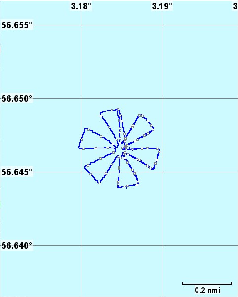
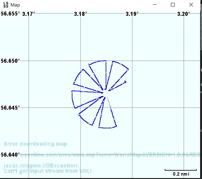
An additional experiment was conducted where Kayak and Otter performed transects around RV Kristine Bonnevie in a flower like pattern (Fig. 5). These transects were conducted to assess whether RV Kristine Bonnevie potential worked as fish attraction device (FAD). During the transects Kayak, Otter and RV Kristine Bonnevie collected acoustic data at all frequencies.
2.2 - HYDROGRAPHICAL DATA
(Thor Klevjer, IMR )
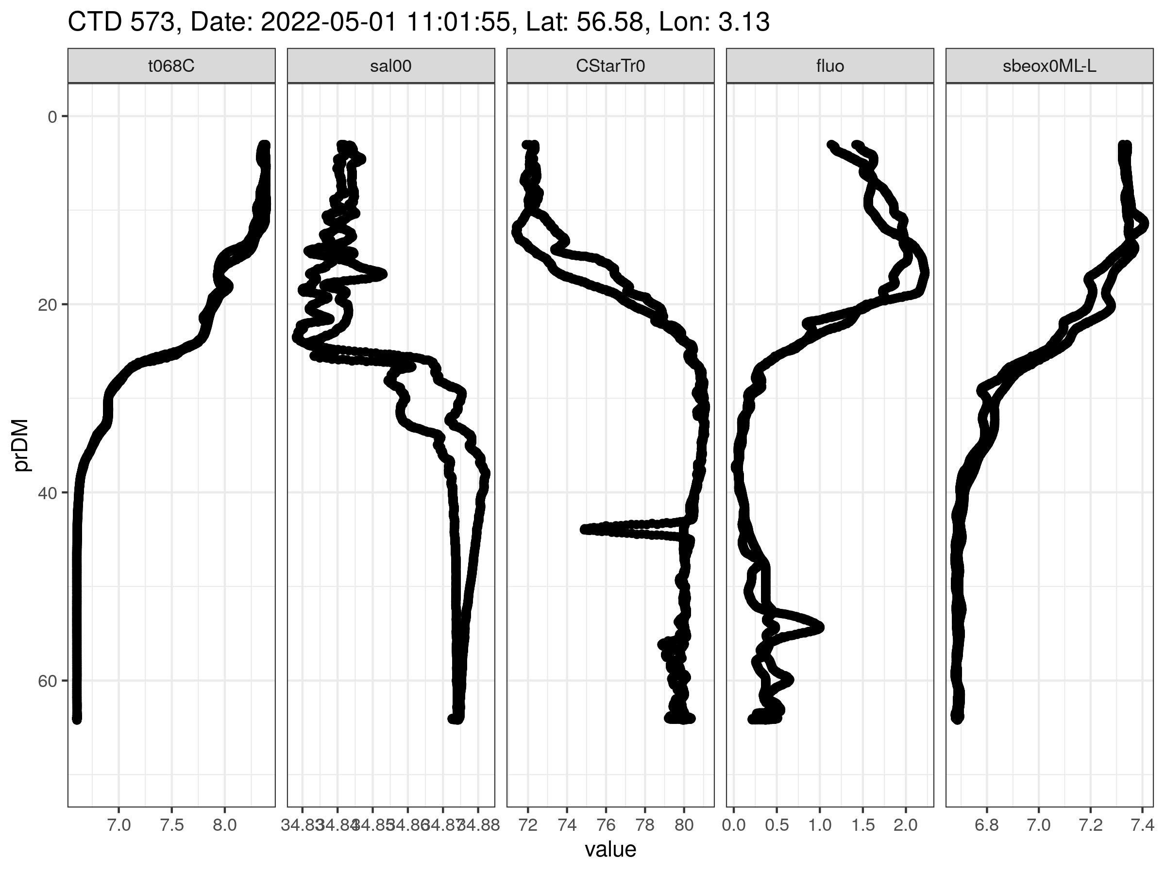
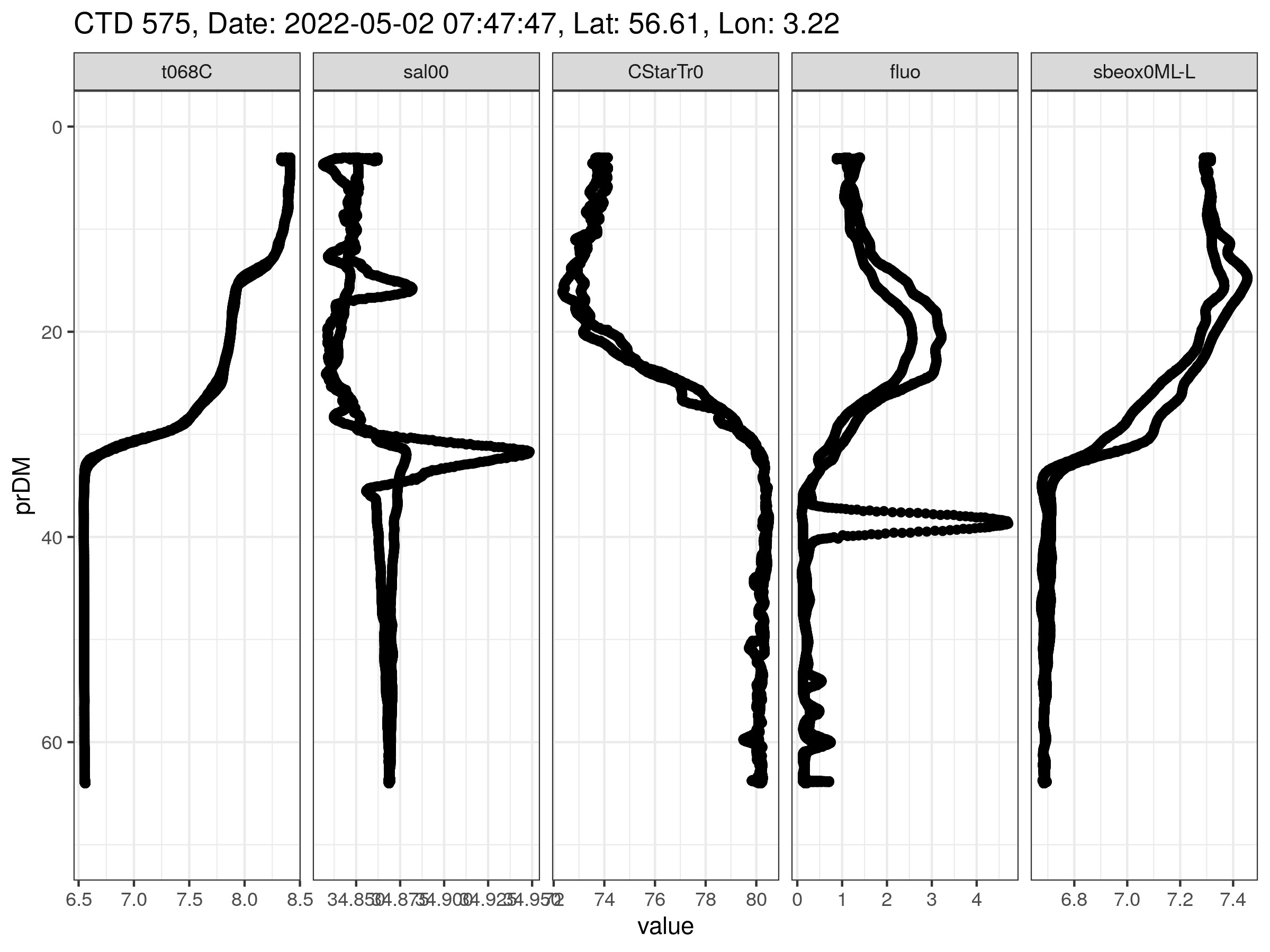
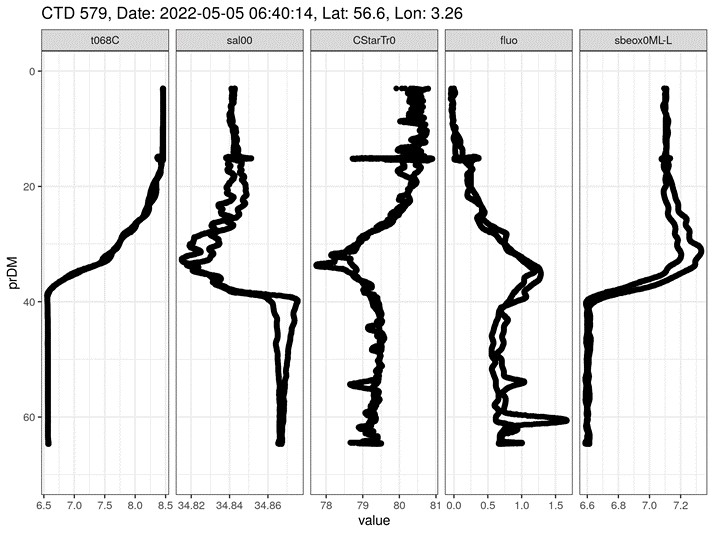
To collect data on the hydrographical conditions at the three WBAT stations and the control station, a CTD (measuring conductivity, temperature and depth) was deployed. The CTD was additionally equipped with a fluorometer (measuring fluorescence), transmissometer (measuring light transmission), oxygen sensor (measuring dissolved oxygen) and also had NISKIN bottles for water sampling, these were used to take samples for chlorophyll and nutrient concentrations.
2.3 - HYDRODYNAMIC MODEL
(Geir Pedersen, IMR)
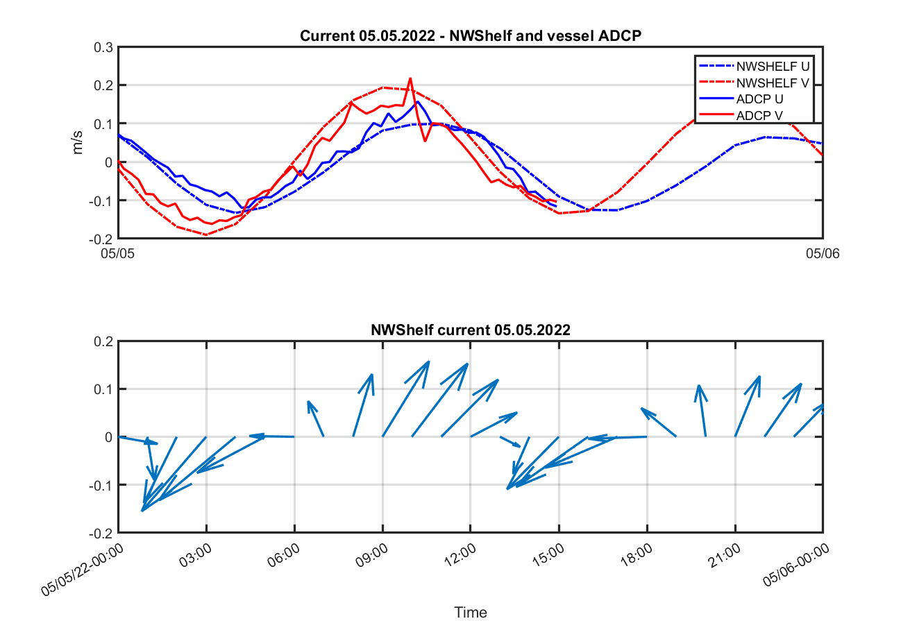
For the daily planning of the main experiments we reviewed multiple data products, and ultimately used the North West Shelf (NWS) oceanographic model predictions of current speed and direction obtained from Copernicus Marine Data Store (NORTHWESTSHELF_ANALYSIS_FORECAST_PHY_004_013). A custom script programmed in Python, using MOTU API, accessed and downloaded the daily predicted speeds and directions in the area where the experiments were taking place. An informal validation of the model predictions is shown in Figure 7 where the predicted U and V component of the current at the surface was compared with measurements from the vessel mounted ADCP (RDI 150 kHz ADCP).
2.4 - PLANKTON SAMPLES
2.4.1 - Quantitative zooplankton samples
(Thor Klevjer, IMR)
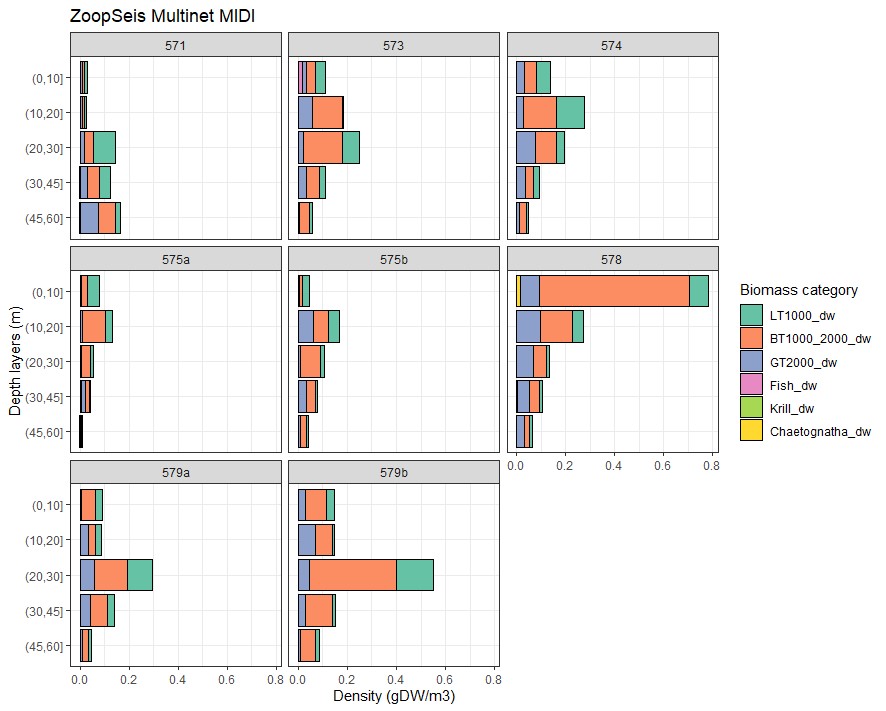
Vertical distributions of zooplankton were estimated through vertical deployments of a 0.25 m2 Hydrobios Multinet equipped with 180 μm mesh size nets, sampling mesozooplankton in the discrete depth intervals 60-45, 45-30, 30-20, 20-10 and 10-0 m. Upon retrieval the nets were washed down on deck, and samples were worked up according to IMR standard protocols. The cod-end samples were split using a Motdo plankton splitter, and half the final sample split (usually the whole sample, but lower splits when large samples) were split in 3 size-fractions (>2 mm, 1-2 mm and 1 mm-180 μm) with sieves, rinsed in freshwater and dried. From the 2 mm fraction important categories according to standard IMR protocols (during this cruise Cheatognaths and fish larvae, and a very few krill and amphipods) were picked, enumerated and dried. The other half of the final sample split was fixed in 4% borax buffered formalin, for later taxonomy, enumeration and staging. On the 3 main stations these multinets were deployed on arrival and at departure, i.e. before and after the nets used for the staining experiments, on the first station (area away from seismic activity) a single multinet was deployed. An additional multinet was deployed at night to assess night-time vertical distribution. On two stations a single 180 μm WP2 net was also deployed from 60-0 m, providing an additional estimate of surface integrated abundances of mesozooplankton.
Echosounder data suggested the presence of fish, in order to sample teleost larvae, we also deployed a WP3 net (1 mm mesh size) vertically from 60-0 m during daytime. Additionally, a single 1m2 Multinet Mammoth (180 μm mesh size) was deployed obliquely, sampling the same vertical strata as the vertical Multinet hauls. These samples were also worked up according to IMR standards.
| Station | Lat | Long | Mon | Day | Time (UTC) | Bottom depth | Station | Sampling | ||||||||
|---|---|---|---|---|---|---|---|---|---|---|---|---|---|---|---|---|
| 571 | 56 ° 40.00 | 03 ° 09.99 | 4 | 30 | 13:14 | 68.0 | Control | CTD | ||||||||
| 571 | 56 ° 40.00 | 03 ° 09.99 | 4 | 30 | 13:19 | 68.0 | Control | WP II | ||||||||
| 571 | 56 ° 40.00 | 03 ° 09.99 | 4 | 30 | 14:04 | 68.0 | Control | Multinet_MIDI, 5 strata sampled | ||||||||
| 572 | 56 ° 40.00 | 03 ° 09.99 | 5 | 1 | 7:25 | 66.7 | Control | CTD | ||||||||
| 573 | 56 ° 35.02 | 03 ° 08.08 | 5 | 1 | 10:32 | 66.7 | WBAT1 | Multinet_MIDI, 5 strata sampled | ||||||||
| 573 | 56 ° 35.02 | 03 ° 08.08 | 5 | 1 | 11:01 | 69.4 | WBAT1 | CTD | ||||||||
| 574 | 56 ° 35.02 | 03 ° 08.08 | 5 | 1 | 16:35 | 69.4 | WBAT1 | Multinet_MIDI, 5 strata sampled | ||||||||
| 575 | 56 ° 36.43 | 03 °13 .49 | 5 | 2 | 7:26 | 69.4 | WBAT2 | Multinet_MIDI, 5 strata sampled | ||||||||
| 575 | 56 ° 36.43 | 03 °13 .49 | 5 | 2 | 7:47 | 68.4 | WBAT2 | CTD | ||||||||
| 575 | 56 ° 36.43 | 03 °13 .49 | 5 | 2 | 13:23 | 68.4 | WBAT2 | Multinet_MIDI, 5 strata sampled | ||||||||
| 577 | 56 ° 36.43 | 03 °13 .49 | 5 | 3 | 6:08 | 69.0 | Control | CTD | ||||||||
| 577 | 56 ° 36.43 | 03 °13 .49 | 5 | 3 | 7:00 | 69.0 | Control | WP II | ||||||||
| 578 | 56 ° 36.13 | 03 °11.21 | 5 | 3 | 20:57 | 68.8 | Control (night) | CTD | ||||||||
| 578 | 56 ° 36.13 | 03 °11.21 | 5 | 3 | 21:19 | 69.0 | Control (night) | Multinet_MIDI, 5 strata sampled | ||||||||
| 578 | 56 ° 36.13 | 03 °11.21 | 5 | 4 | 8:38 | 69.0 | Control | WP3 | ||||||||
| 579 | 56 ° 36.12 | 03 °15.48 | 5 | 5 | 6:40 | 69.0 | WBAT3 | CTD | ||||||||
| 579 | 56 ° 36.12 | 03 °15.48 | 5 | 5 | 7:28 | 69.0 | WBAT3 | Multinet_MIDI, 5 strata sampled | ||||||||
| 579 | 56 ° 36.12 | 03 °15.48 | 5 | 5 | 13:32 | 69.0 | WBAT3 | Multinet_MIDI, 5 strata sampled | ||||||||
| 579 | 56 ° 36.12 | 03 °15.48 | 5 | 5 | 16:53 | 69.0 | WBAT3 | Multinet_MAMMOTH, 5 strata sampled | ||||||||
2.4.2 - Discrimination of live and dead zooplankton:
(Josefin Titelman, University of Oslo)
Zooplankton mortality was analyzed from samples from vertical net tows (WP2) taken at different distances from the seismic shooting (Table 4). Samples were stained with a live stain and photographed (Elliott and Tang 2009). At all times dead controls were also stained. Images will be analyzed using an automated procedure that efficiently assigns each copepod to either live or dead. Preliminary scanning by eye suggests limited (if any) effects of the seismic activity.
| Purpose | Date | Position | CTD station | Animals | Stain conc. (ml stock/L) | Staining time (min) | Killing method |
|---|---|---|---|---|---|---|---|
| WBAT1 | 1 May | 56 ° 35.02N 03 ° 08.08E | 573 | WP2 (0-60m) | 0.3/1 | 15 | Fresh water 3 min |
| WBAT2 | 2 May | 56 ° 36.43N 03 ° 13.49E | 575 | WP2 (0-60m) | 0.3/1 | 15 | Fresh water 5 min |
| WBAT3 | 5 May | 56 ° 36.12N 3 ° 15.48E | 579 | WP2 (0-60) | 1.5/1 | 15 | Heat, 40 °C 10 min |
| Control | 3 May | 56 ° 36.13N 03 ° 11.21 E | 578 | WP2, 0-58m | 1.5/1 | 15 | Heat 40 °C 10 min |
| Bags 1, instant mortality | 3 May | 56 ° 36.13N 03 ° 11.21 E | NA | From WP2 | 1.5/1 | 15 | Heat 40 °C 10 min |
| Bags 2, instant mortality | 4 May 10:45-13:32 | 56 ° 36.477N 03 ° 12.301E | NA | From WP2 | 1.5/1 | 15 | Heat 40 °C * 10min |
| Bags 3, instant mortality | 4 May 15:35-16:35 | 56 ° 36.476N 03 ° 12.402E | NA | From WP2 | 1.5/1 | 15 | Heat 40 °C * 10min |
| Test staining time | 4 May | NA | NA | From WP2 | 1.5/1 | 15, 30, 60, 120 | Heat 40 °C 10min |
| * Dead controls from “Staining time”, at 15 min, conducted in the same photo session | |||||||
| WP2 number | Dato | SS | LocID | Depth | Start_UTC | Stop_UTC | ES_guess |
|---|---|---|---|---|---|---|---|
| 1 | 30/4/2022 | 572 | A | 7:36:00 | TEST | ||
| 2 | 30/4/2022 | 572 | B | 7:43:00 | TEST | ||
| 3 | 1/5/2022 | 573 | A | 60 | 13:21:45 | 13:23:32 | WBAT1 |
| 4 | 1/5/2022 | 573 | DEAD | 35 | 13:25:00 | 13:27:00 | WBAT1 |
| 5 | 1/5/2022 | 573 | B | 60 | 13:34:55 | 13:36:55 | WBAT1 |
| 6 | 1/5/2022 | 573 | C | 60 | 13:50:01 | 13:52:05 | WBAT1 |
| 7 | 1/5/2022 | 573 | D | 60 | 14:05:00 | 14:08:08 | WBAT1 |
| 8 | 1/5/2022 | 573 | E | 60 | 14:11:45 | 14:13:47 | WBAT1 |
| 9 | 1/5/2022 | 573 | F | 60 | 14:17:06 | 14:18:59 | WBAT1 |
| 10 | 1/5/2022 | 573 | G | 60 | 14:22:04 | 14:24:00 | WBAT1 |
| 11 | 1/5/2022 | 573 | H | 60 | 14:27:11 | 14:29:08 | WBAT1 |
| 12 | 1/5/2022 | 573 | I | 60 | 14:45:26 | 14:47:26 | WBAT1 |
| 13 | 1/5/2022 | 573 | J | 60 | 14:50:50 | 14:52:36 | WBAT1 |
| 14 | 1/5/2022 | 573 | K | 60 | 14:55:25 | 14:57:25 | WBAT1 |
| 15 | 1/5/2022 | 573 | L | 60 | 15:00:20 | 15:02:16 | WBAT1 |
| 16 | 1/5/2022 | 573 | M | 60 | 15:05:05 | 15:07:10 | WBAT1 |
| 17 | 2/5/2022 | 575 | A | 60 | 10:15:00 | 10:17:00 | WBAT2 |
| 18 | 2/5/2022 | 575 | B | 60 | 10:30:00 | 10:32:30 | WBAT2 |
| 19 | 2/5/2022 | 575 | C | 60 | 10:45:00 | 10:47:08 | WBAT2 |
| 20 | 2/5/2022 | 575 | D | 60 | 11:00:00 | 11:02:05 | WBAT2 |
| 21 | 2/5/2022 | 575 | E | 60 | 11:15:00 | 11:17:05 | WBAT2 |
| 22 | 2/5/2022 | 575 | F | 60 | 11:30:00 | 11:32:15 | WBAT2 |
| 23 | 2/5/2022 | 575 | G | 60 | 11:45:00 | 11:46:55 | WBAT2 |
| 24 | 2/5/2022 | 575 | H | 60 | 11:55:00 | 11:57:20 | WBAT2 |
| 25 | 2/5/2022 | 575 | I | 60 | 12:00:00 | 12:02:10 | WBAT2 |
| 26 | 2/5/2022 | 575 | J | 60 | 12:04:35 | 12:06:30 | WBAT2 |
| 27 | 2/5/2022 | 575 | K | 60 | 12:09:15 | 12:11:10 | WBAT2 |
| 28 | 2/5/2022 | 575 | L | 60 | 12:13:45 | 12:15:45 | WBAT2 |
| 29 | 2/5/2022 | 575 | M | 60 | 12:18:20 | 12:20:05 | WBAT2 |
| 30 | 2/5/2022 | 575 | N | 60 | 12:22:30 | 12:24:32 | WBAT2 |
| 31 | 2/5/2022 | 575 | O | 60 | 12:27:19 | 12:29:15 | WBAT2 |
| 32 | 3/5/2022 | 577 | A | 58 | 7:10:00 | 7:12:00 | STAINING CONTROLS |
| 33 | 3/5/2022 | 577 | B | 58 | 7:35:15 | 7:37:08 | STAINING CONTROLS |
| 34 | 3/5/2022 | 577 | C | 58 | 7:40:32 | 7:42:25 | STAINING CONTROLS |
| 35 | 3/5/2022 | 577 | D | 58 | 7:46:20 | 7:48:17 | STAINING CONTROLS |
| 36 | 3/5/2022 | 577 | Dead 1 | 58 | 7:51:40 | 7:53:26 | STAINING CONTROLS |
| 37 | 3/5/2022 | 577 | Dead2 | 58 | 7:57:55 | 7:59:45 | STAINING CONTROLS |
| 38 | 3/5/2022 | 577 | Dead3 | 58 | 8:03:15 | 8:05:08 | STAINING CONTROLS |
| 39 | 5/4/2022 | 578 | A | 58 | 13:05:00 | 13:07:00 | STAINING CONTROLS |
| 40 | 5/4/2022 | 578 | B | 58 | 13:11:00 | 13:13:00 | STAINING CONTROLS |
| 41 | 5/4/2022 | 578 | C | 58 | 13:17:00 | 13:19:00 | STAINING CONTROLS |
| 42 | 5/5/2022 | 579 | A | NA | 11:40:40 | 11:42:40 | WBAT3 |
| 43 | 5/5/2022 | 579 | B | NA | 11:55:00 | 11:57:00 | WBAT3 |
| 44 | 5/5/2022 | 579 | C | NA | 12:10:00 | 12:12:00 | WBAT3 |
| 45 | 5/5/2022 | 579 | D | NA | 12:15:15 | 12:17:30 | WBAT3 |
| 46 | 5/5/2022 | 579 | E | NA | 12:20:00 | 12:22:00 | WBAT3 |
| 47 | 5/5/2022 | 579 | F | NA | 12:24:50 | 12:27:15 | WBAT3 |
| 48 | 5/5/2022 | 579 | G | NA | 12:30:05 | 12:32:05 | WBAT3 |
| 49 | 5/5/2022 | 579 | H | NA | 12:35:10 | 12:37:05 | WBAT3 |
| 50 | 5/5/2022 | 579 | I | NA | 12:40:00 | 12:42:02 | WBAT3 |
| 51 | 5/5/2022 | 579 | J | NA | 12:44:50 | 12:47:05 | WBAT3 |
2.5 - PLANKTON EXPERIMENTS - SURVIVAL
2.5.1 - Bag experiments – methods
(Emilie Hernes Vereide, IMR and University of Oslo)
Preparation
Live cultured Calanus finmarchicus were kept at 10ºC in a container, 25 L buckets with filtered water.
2.5.1.1 - Calanus bags
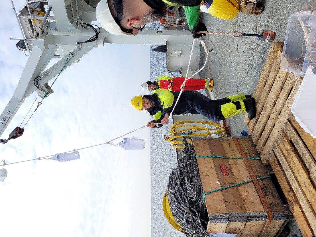
We carefully transferred 10 cultured Calanus finmarchicus to 1L ziplock plastic bags, holding filtered seawater at a temperature of 10ºC. Further, we placed each plastic bag in nylon netting bag (laundry bags). Then 3 netting bags, holding 10 copepods each, were tied onto a line and lowered to the water. For every transect, 1 line was deployed at the very beginning, and four lines were deployed the last 8 minutes, or as close as possible to the seismic vessel. For every line, the bags were lowered to a depth of 10 m, kept there for 15 seconds, before pulled up (Fig 9).
Here, one control of no shooting was conducted, in addition to 3 rounds of exposure (3 WBAT transects). Also, we had one semi control Saturday 30th of April, with shooting from a far distance.
After deployment, every individual C. finmarchicus was investigated live/dead and transferred to 50 mL bottles for further investigations of delayed mortality. Dead individuals were taken out and photographed to determine size and stage. The bottles were kept in the container at 10ºC.
2.5.1.2 - Wild zooplankton
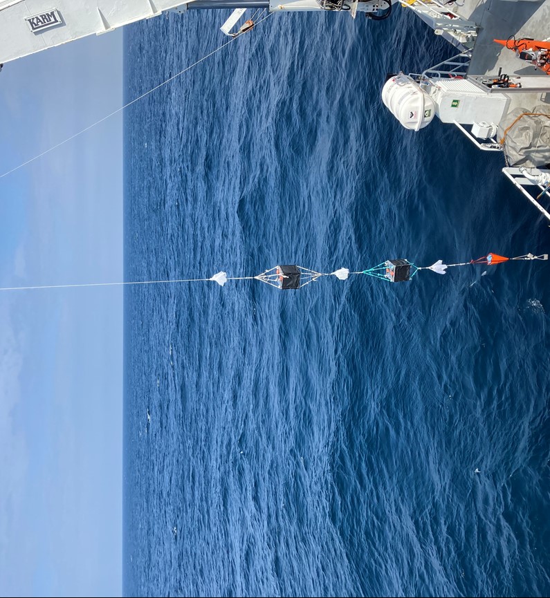
Net hauls (WP2) were taken Tuesday 3rd of May, when there was no shooting in the area. The zooplankton were kept in 25 L buckets at 10ºC with light aeration. Bulks of the sample were put in bags and attached to a line along with the zooplankton cages (2.5) for 1 hour of deployment (Figure 10). Here, one control with no shooting was conducted, in addition to 3 rounds with exposure. After exposure, the zooplankton were stained to determine mortality.
| Date | Treatment | Cultured/wild | # Lines per approach | # bags per line | # animals per bag | Time in water | Description |
|---|---|---|---|---|---|---|---|
| 30.04.2022 | Control (3nm) | Cultured | 4 | 3 | 10 | 45s | |
| 01.05.2022 | WBAT1 transect | Cultured | 5 | 3 | 10 | 45s | 1 line at furthest distance, 4 lines last 8 min before passage |
| 01.05.2022 | Picking control | Cultured | 1 | 6 | 10 | - | Stayed in container |
| 02.05.2022 | WBAT2 transect | Cultured | 5 | 3 | 10 | 45s | 1 line at furthest distance, 4 lines last 8 min before passage |
| 02.05.2022 | Picking control | Cultured | 1 | 6 | 10 | - | Stayed in container |
| 03.05.2022 | Control no shooting | Cultured | 4 | 3 | 10 | 45s | |
| 03.05.2022 | Control no shooting | Wild | 4 | 3 | > 100 | 45s | On same lines as above |
| 04.05.2022 | Passage | Wild | 1 | 12 | > 100 | 60 min | From far to close passage, on cage |
| 04.05.2022 | Passage | Wild | 1 | 12 | > 100 | 60 min | From far to close passage |
| 05.05.2022 | WBAT3 transect | Cultured | 5 | 3 | 10 | 45s | 1 line at furthest distance, 4 lines last 8 min before passage |
| 05.05.2022 | Picking control | Cultured | 1 | 6 | 10 | - | Stayed in container |
| 05.05.2022 | WBAT3 transect | Cultured | 1 | 4 | 50 | 45s | 50 individuals per bags |
| 05.05.2022 | WBAT3 transect | Wild | 1 | 6 | > 100 | 40 min | At stat of transect, On cage |
| 05.05.2022 | Picking control | Wild | 1 | 6 | > 100 | - | Stayed in container |
2.6 - COPEPOD BEHAVIOUR
(Saskia Kühn, Kiel University, Coastal Ecology Research and Technology Centre West Coast Büsum)
In this experiment we have exposed wild caught zooplankton, cultured adult Calanus finmarchicus, to real-time seismic air gun blasts. Copepod behavior was filmed and will be analyzed before, during and between the exposures.
Cage experiment
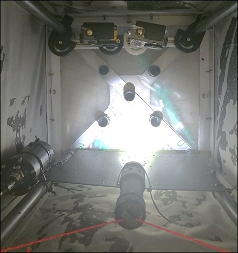
Two 40*40*40 cm cages, based on an aluminum frame enclosed with a 100 µm mesh net and a black plastic bag to darken the cage, were each equipped with a stereo-camera setup (Figure 11). The cameras were pointing towards a black PVC plate on which a white diving light was connected. The two cages were connected with a rope so that one cage was 2 meters on top of the other cage (Figure 10). The upper cage was connected to a buoy with a 10 m long rope. We connected a floating plus weights to the lower cage in order to stabilize the setup. After the preparation of the setup we put 100 copepods into a small holding tanks inside the cages. The holding tank opened automatically when the cages were lowered into the water, and released the experimental animalssmall to the cages. Then, the lights and cameras were turned on. The setup was thereafter put into the water with a crane and stayed there for approximately 1 hour. The 1 hour was chosen to study the animal behavior during increasing seismic exposure (during an a approach of the seismic vessel). We timed the deployment so that the seismic ship would pass exactly after 60 minutes of deployment. Beside the exposure we additionally included controls at times without any shooting from the seismic ship. The data will be analyzed upon individual copepod behavior (see Table 6).
| Date | Code | Control/ Exposure | Cage | Copepods Culture/ Wild | Num. of Copepods | Time IN | Time OUT | Comments |
|---|---|---|---|---|---|---|---|---|
| 01.05.2022 | ZS_1 | Control | 1 | Culture | 100 | 08:15 | 09:15 | All times from watch Saskia Kühn Synchronized at klokka.no |
| 02.05.2022 | ZS_2 | Exposure | 1 | Culture | 100 | 14:42 | 15:12 | |
| 03.05.2022 | ZS_3 | Control | 1 | Wild | 100 | 12:36 | 13:36 | |
| 03.05.2022 | ZS_4 | Control | 2 | Wild | 100 | 12:36 | 13:36 | |
| 03.05.2022 | ZS_5 | Control | 1 | Wild | 100 | 16:15 | 17:15 | |
| 04.05.2022 | ZS_6 | Exposure | 1 | Culture | 100 | 12:38 | 13:45 | |
| 04.05.2022 | ZS_7 | Exposure | 2 | Culture | 100 | 12:38 | 13:45 | |
| 04.05.2022 | ZS_8 | Exposure | 1 | Culture | 100 | 17:39 | 18:45 | |
| 04.05.2022 | ZS_9 | Exposure | 2 | Culture | 100 | 17:39 | 18:45 | |
| 05.05.2022 | ZS_10 | Exposure | 1 | Culture | 100 | 13:56 | 14:50 | |
| 05.05.2022 | ZS_11 | Exposure | 2 | Culture | 100 | 13:56 | 14:50 | |
| 06.05.2022 | ZS_12 | Control -Exposure | 1 | Culture | 130 | 11:49 | 12:35 | |
| 06.05.2022 | ZS_13 | Control - Exposure | 2 | Culture | 130 | 11:49 | 12:35 |
2.7 - HYDROPHONE DATA
(Karen de Jong, IMR)
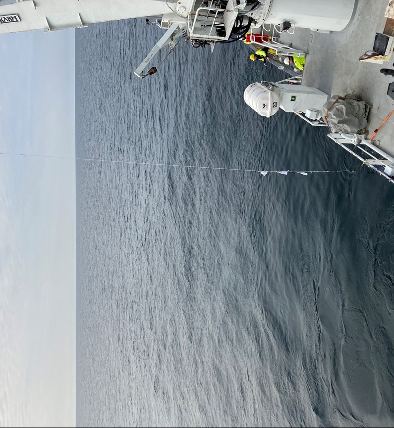
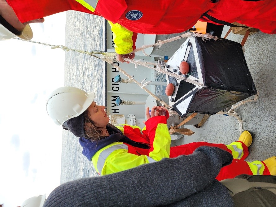
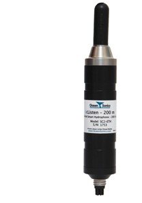
To measure ambient sound and the sound from the seismic survey, we deployed an Ocean Sonic Eth-X2 hydrophone (sensitivity 205 dB re 1 µPa) (Figure 12 topp) on a rope midships from the port side of the research vessel. The hydrophone was deployed on a steel bracket hanging from a rope at 10m depth. The hydrophone recorded while the seismic ship was approaching and at three occasions it recorded until it had passed.
| Date | Time start (UTC) | Time stop (UTC) | Approximate time of passage* | Description |
|---|---|---|---|---|
| 30.04.2022 | 17:57:50 | 18:13:46 | Control station (no passage) | |
| 01.05.2022 | 08:32:00 | 10:47:00 | Control station (no passage) | |
| 01.05.2022 | 13:10:00 | 14:31:15 | 14:56 | WBAT1 transect |
| 02.05.2022 | 09:20:00 | 12:06:10 | 12:12 | WBAT2 transect |
| 03.05.2022 | 12:26:00 | 13:00:00 | Control on site without shooting | |
| 04.05.2022 | 10:55:04 | 11:50:00 | 10:37 | Extra pass |
| 04.05.2022 | 15:47:00 | 16:36:00 | 16:36 | Pass on port side |
| 05.05.2022 | 11:42:00 | 12:36:00 | 12:34 | WBAT3 transect |
| 06.05.2022 | 11:47:00 | 12:30:00 | 12:27 | Pass at the start of a shooting transect, port side, hydrophone in water before shooting started. |
* Taken from when last bags were taken out of the water
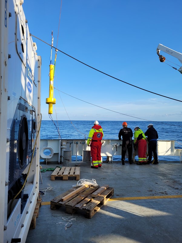
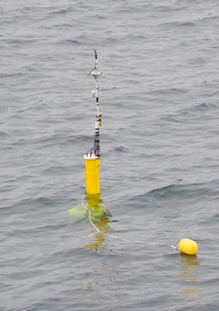
In addition, an anti-heave surface buoy with a vertical hydrophone array (Figure 12 middel and bottom) was deployed on northern end of the Ekofisk area, close to the position of WBAT 3. This buoy contained an UNO-2483G embedded computer with an internal flash drive for data-logging and instrumentation control and two calibrated omnidirectional hydrophones (Naxys 02345, frequency range: 5 Hz to 300 kHz, sensitivity: -179 dB re V/μPa) hydrophones that can be deployed at variable depths. One of the hydrophones was deployed at 8 m depth (sampling rate: 96 kHz, gain 0 dB) and one at 35 m depth (768 kHz, gain: 0 dB). The hydrophones recorded from 3.5.2022 17:50 till 04.05.2022 16:57:41, with a duty cycle of 28s on, 2s off. A GPS receiver enabled the buoy to be tracked and a radio Ethernet link allowed remote control and monitoring of the system. The GPS position were logged to document the exact location of the buoy over the 24-hours deployment period.
In addition to these two hydrophones we deployed a hydrophone glider, Slocum, for Akvaplan-niva on the 30th of May. Ambient sound record will also be provided from a lander rigged with JASCO hydrophone deployed at Ekofisk in March 2022 and will be retrieved in March 2023 (position of lander: Long: 3.171969 - Lat: 56.537685 (WGS 84)).
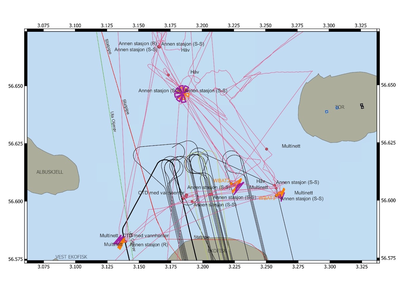
2.8 - ACTIVITY MAP
Below (Figure 13) is a map showing the cruise activity at Ekofisk. Tracking both Kristine Bonnevie and the seismic vessel Skandi Nova from the 30th of April to the 6th of May. Two of the WBAT stations (WBAT 2 and 3) are marked by name in orange. WBAT 1 is located west in the shooting area where you see the dens tracks of the kayak (orange) and Otter (purple). We had two control stations, one ca 5 nm to the north (the most northern stations on the map) and one control station between WBAT1 and WBAT2. The FAD station was North of the shooting area, between the two control stations visible as a flower track. For latitude and longitude position see Table 2, for date and time see Table 7.
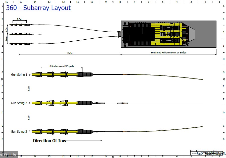
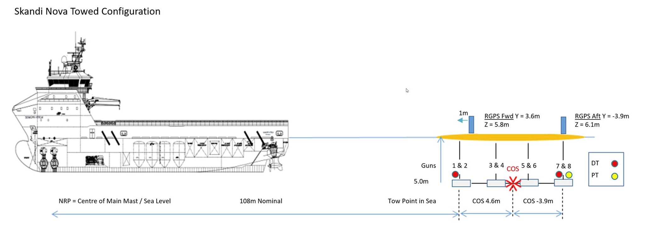
2.9 - SEISMIC AIRGUN
Below (Table 8) follows a description of the properties and positioning of the seismic air gun used in the experiment.
| Source Parameters | |
|---|---|
| Number of Sources | 1 |
| Number of Sub-Arrays (Strings) per Source | 3 |
| Array Length | 8.55 m |
| Sub-Array Separation | 6 m |
| Source Width | 12 m |
| Source Wolum | 3060 Cubic inches |
| Number of Hydrophones per String | 4 |
| Number of Depth Transducers per String | 3 |
| Number of Pressure Transducers per String | 1 |
| Number of Guns per String (all Clusters) | String 1 = 8 (4 Clusters) |
| String 2 = 8 (4 Clusters) | |
| String 3 = 8 (4 Clusters) | |
| Airgun Type | Sercel G-Gun II |
| Operating Pressure | 2000 PSI |
| Depth of Guns | 5.0 m +/- 0.5 m |
| Peak to Peak Amplitude | 82.06 bar m |
| Primary to Bubble Ratio | 29.14 |
3 - Referances
Bickel SL, Malloy Hammond, JD, and Tang, KW. (2011). Boat-generated turbulence as a potential source of mortality among copepods. Journal of Experimental Marine Biology and Ecology 401:105-109. doi.org/10.1016/j.jembe.2011.02.038
Booman C, Dalen J, Leivestad H, Levsen A, van der Meeren T, and Toklum K. (1996). Effekter av luftkanonskyting på egg, larver og yngel. Undersøkelser ved Havforskningsinstituttet og Zoologisk Laboratorium, Universitetet i Bergen. Fisken og Havet, 3:83s
Elliott, DT and Tang, KW, Simple staining method for differentiating live and dead marine zooplankton in field samples (2009). Limnology And Oceanography-Methods, 7:585-594. doi:10.4319/lom.2009.7.585
Fields D, Handegard NO, Dalen J, Malde K, Karlsen Ø, Skiftesvik AB, Durif C, and Browman H. (2019). Airgun blast used in marine geological surveys have a minor effect on survival at distances less than 10 m and no sub-lethal effects on behaviour and gene expression in the copepod Calanus finmarchicus. Ices Journal of Marine ScienceICES Journal of Marine Science, doi:10.1093/icesjms/fsz126
McCauley RD, Day RD, Swadling KM, Fitzgibbon QP, Watson RA, and Semmens JM. (2017). Widely used marine seismic survey air gun operations negatively impact zooplankton, Nature Ecology & Evolution 1: 0195. doi: 10.1038/s41559-017-0195
Nedelec SL, Simpson SD, Morley EL, Nedelec B, Radford AN (2015). Impacts of regular and random noise on the behaviour, growth and development of larval Atlantic cod (Gadus morhua). Proceedings of the Royal Society B 282:20151943. doi:10.1098/rspb.2015.1943
Tang KW, Ivory JA, Shimode S, Nishibe Y, and Takahashi K, (2019). Dead heat: copepod carcass occurrence along the Japanese coasts and implications for a warming ocean. ICES Journal of Marine Science 76:1825–1835. doi:10.1093/icesjms/fsz017