Management strategy evaluation for northern shrimp in the Barents Sea (ICES subareas 1 and 2)

1.1 - Request summary

The need to establish a management plan for the shrimp fishery in ICES areas I and II has been discussed in the Joint Norwegian-Russian Fisheries Commission (JNRFC) in both 2021 and 2022. In 2023, the JNRFC requested the development and evaluation of harvest control rules (HCR) for shrimp as priority. The results are to be presented at the meeting of the JNRFC in October 2024 to decide on the adoption of a new HCR, to be applied as basis for the total allowable catch (TAC) of the stock in 2025.

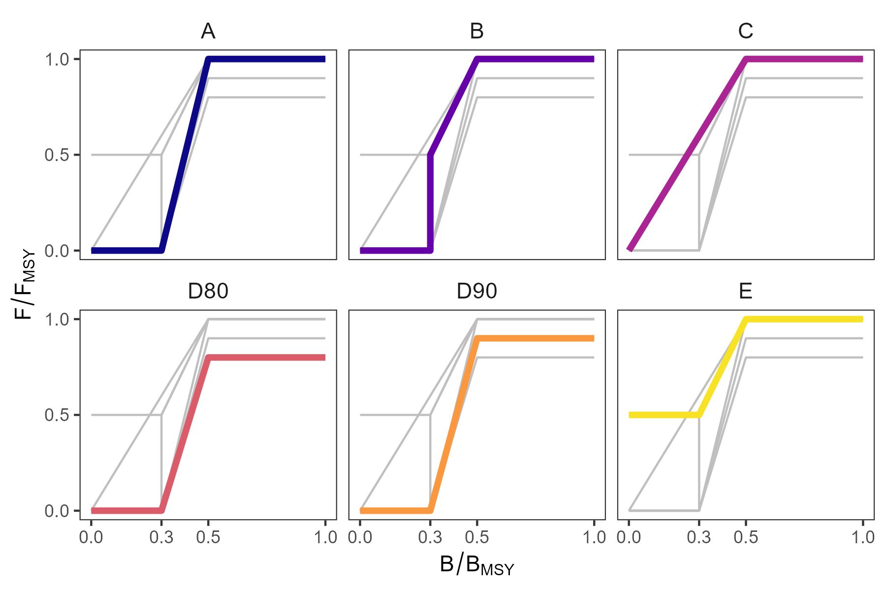
In the first half of 2023, the Institute of Marine Research (IMR) developed a Management Strategy Evaluation framework (MSE) to investigate possible HCRs. The Directorate of Fisheries organized a meeting on 4 July 2023 between the Ministry of Business and Fisheries, IMR and the Directorate of Fisheries, where HI presented the shrimp MSE framework and discussed various alternative HCRs to test. This was followed by a stakeholder meeting on 29 August 2023 between the Institute of Marine Research, Directorate of Fisheries, and industry representatives from Fiskarlaget, Fiskebåt, Sjømat Norge and Norges Råfisklag to present the MSE framework and candidate HCRs. At this meeting, it was agreed that the proposed MSE framework would be used to evaluate the consequences of a set of alternative HCRs (Figure 1), defined as follows:

• HCR A: F is set equal to F_MSY when biomass is above B_trigger and reduced linearly from F_MSY at B_trigger to 0.0 at biomass equal to B_lim.

• HCR B: Like HCR A, but F is reduced linearly from F_MSY at B_trigger to 0.5 F_MSY at B_lim, and then directly to 0.0 when below B_lim.

• HCR C: Like HCR A, but F is reduced linearly from F_MSY at B_trigger to 0.0 at biomass equal to 0.0.

• HCR D80 and D90: Like HCR A, but F_target is set to a) 80% of F_MSY (D80) or b) 90% of F_MSY (D90).

• HCR E: Like HCR B, but where F remains at 50% of F_MSY when bioamss is below B_lim.

B_trigger and B_lim were defined relative to the biomass that produces maximum sustainable yield as B_trigger = 0.5 B_MSY and B_lim = 0.3 B_MSY, whereas F_target was defined as either equal to the fishing mortality producing maximum sustainable yield, F_MSY, or a fraction thereof, depending on the HCR. All HCRs include a catch constraint that limits changes in total allowable catch (TAC) from year to year to +20%/-20%.

Per agreement, all HCRs were evaluated based on three main performance criteria:

1. The probability of SSB falling below B_lim in any single year should not exceed 5%.

2. High long-term yield should be achieved in respect to median long-term yield attained by fishing at the deterministic F_MSY.

3. Median biomass should be above B_MSY.

The performance of the HCRs were assessed in a short- (5 years), medium-(10 years), and long-term (40 years) perspective. In addition to the main performance criteria, the following metrics were considered: probability of biomass falling below B_trigger; biomass relative to B_MSY; F relative to F_MSY; mean relative change in TAC from year to year. In response to requests on evaluating the robustness of HCRs against potential ecosystem shifts, all HCRs were tested against a scenario where the underlying productivity of the stock is reduced. The low productivity scenario was modelled by reducing the carrying capacity by 50%, simulating a regime shift towards lower ecosystem productivity due to e.g. climate change.

2.1 - Overview

The MSE framework for shrimp in the Barents Sea was developed using the framework described in Punt et al. (2016). In general, an MSE is a closed-loop simulation where all feedbacks between management, fishing, and fish biology are captured by and linked through mathematical models. These models typically include an: 1. operating model, which simulates the ‘true’ population dynamics and the fishery; 2. observation model, which generates survey and catch information by simulating the sampling and fishery of the true population abundances with observation error; 3. estimation model, which uses the generated data from the operating model as input for a stock assessment model to estimate stock size and parameters from the simulated data; 4. decision model, which uses the estimates and forecasts (e.g. biomass) from the estimation model to compute a target exploitation rate (e.g. fishing mortality) via a harvest control rule (HCR), and translates this target to the actual advice value (e.g. TAC); 5. implementation model, which converts the management advice (TAC) to the actual catch taken from the ‘true’ population (i.e. with or without error).

The catches projected from the implementation model are fed into the operating model, and this model sequence is repeated over many years. The estimation and decision models together form the management procedure, while the observation and implementation models may be considered part of the operating model (Punt 2016). Furthermore, different starting population abundances, random errors, and parameter values should be used to simulate different iterations of potential population dynamics and fishing trajectories. Simulating many different trajectories aims at capturing the different sources of uncertainty, especially future recruitment variability and errors in monitoring data. Finally, performance metrics are computed from all simulated trajectories to quantify across iterations how well each management procedure meets management objectives, such as maximizing yield and minimizing risk.

A key purpose of MSE is to test the robustness of management strategies against uncertainty, as measured by the pre-defined performance metrics. Uncertainty can and should be represented by using different operating models in addition to different parameter values and randomly generated errors used in each iteration of the MSE simulations. Alternative operating models may include “worst-case” or other alternative scenarios that are configured and conditioned based on expert judgment and additional/ancillary information. With each different operating model, the MSE loop is re-run with a different set of iterations and the performance statistics are re-calculated. Generally, one baseline operating model is used as the most ‘realistic’ scenario, which all possible management strategies are tested against. Alternative operating models may represent other plausible or even pessimistic scenarios and used to test all or a candidate subset of strategies.

We used the ‘mse’ package available in FLR (https://github.com/flr/mse) to develop and run the code for the shrimp MSE. The ‘mse’ package has been used to code and run other MSEs to fulfill HCR requests for ICES stocks (ICES 2019a, ICES 2019b) and for which R scripts are often made publicly available on Github. The ‘mse’ package is part of the FLR collection of libraries (Kell 2007), which has built-in tools to condition and flexibly parameterize each model of the MSE, easily setup a variety of pre-configured stock assessment models for the MSE estimation model and contains pre-configured ICES standard HCRs for use in the decision model. The scripts used for the MSE are available at https://github.com/FBZimmermann/NEAshrimpMSE.

2.2 - Baseline operating model (OM1)

2.2.1 - Model and settings

The structure of the baseline operating model OM1 was based on the current stock assessment for shrimp in the Barents Sea (Hvingel and Zimmermann 2024). The assessment uses SPiCT, a continuous-time surplus production model that is fitted to time series of catches and stock indices (here standardized survey and commercial CPUE indices) to estimate the parameters of a generalized state-space surplus production model (Pedersen and Berg 2017, Berg 2021). A discrete annual time-step is used for projection with OM1, in contrast to the sub-annual time steps used within the stochastic differential equations of SPiCT. An annual time-step avoids assuming an arbitrary process model for fishing, whereas SPiCT forces a seasonal structure or pattern on fishing. Projections are started from the most recent assessment year (2023).

2.2.2 - Surplus production model

The population dynamics of OM1 are generally modelled by two components: 1) an equation that updates the biomass from year to year and 2) an equation that computes biomass surplus production based on the intrinsic growth rate (r) and carrying capacity (K) of the population (example curves from these components shown in Figure 2). Interannual changes in biomass are the sum of biomass in the current year, the total annual removal of biomass due to catches, and a surplus production term. For surplus production, a stable parameterization (Fletcher 1978) of the generalized Pella-Tomlinson model (Pella and Tomlinson 1969) was used. The Fletcher version of the production equation avoids direct estimation of r since it is highly correlated with K. The growth rate r can be derived from the alternative parameters that are estimated in this model. The parameter values for this model are based on the parameter distributions estimated in the stock assessment.

2.2.3 - Parameter uncertainty

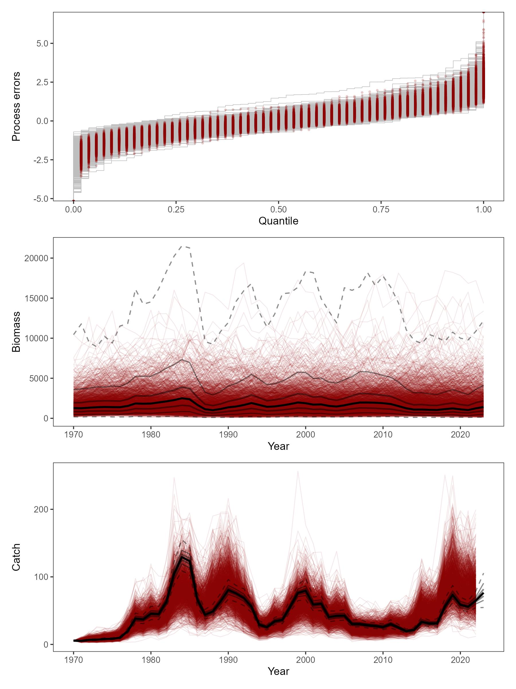
To include parameter uncertainty for OM1, we used the variance-covariance matrix of the fixed effect parameter vector from SPiCT fit of the 2023 assessment to simulate new parameter vectors from a multivariate normal distribution (Figure 3). A unique parameter vector was generated for each iteration of the MSE. SPiCT also estimates process noise to account for other factors (e.g. environmental drivers) that are not intrinsic to the production model, and a similar model was included in OM1 to simulate future process errors. To condition a process error simulation model, we first computed annual production terms for the historical period using SPiCT estimated biomasses at the start of each year and annual catches. The historical annual process errors were then calculated as the difference between these annual production estimates and the annual production predicted from the Fletcher surplus production equation, using the starting biomass of each year (Figure 4).

2.2.4 - Process error

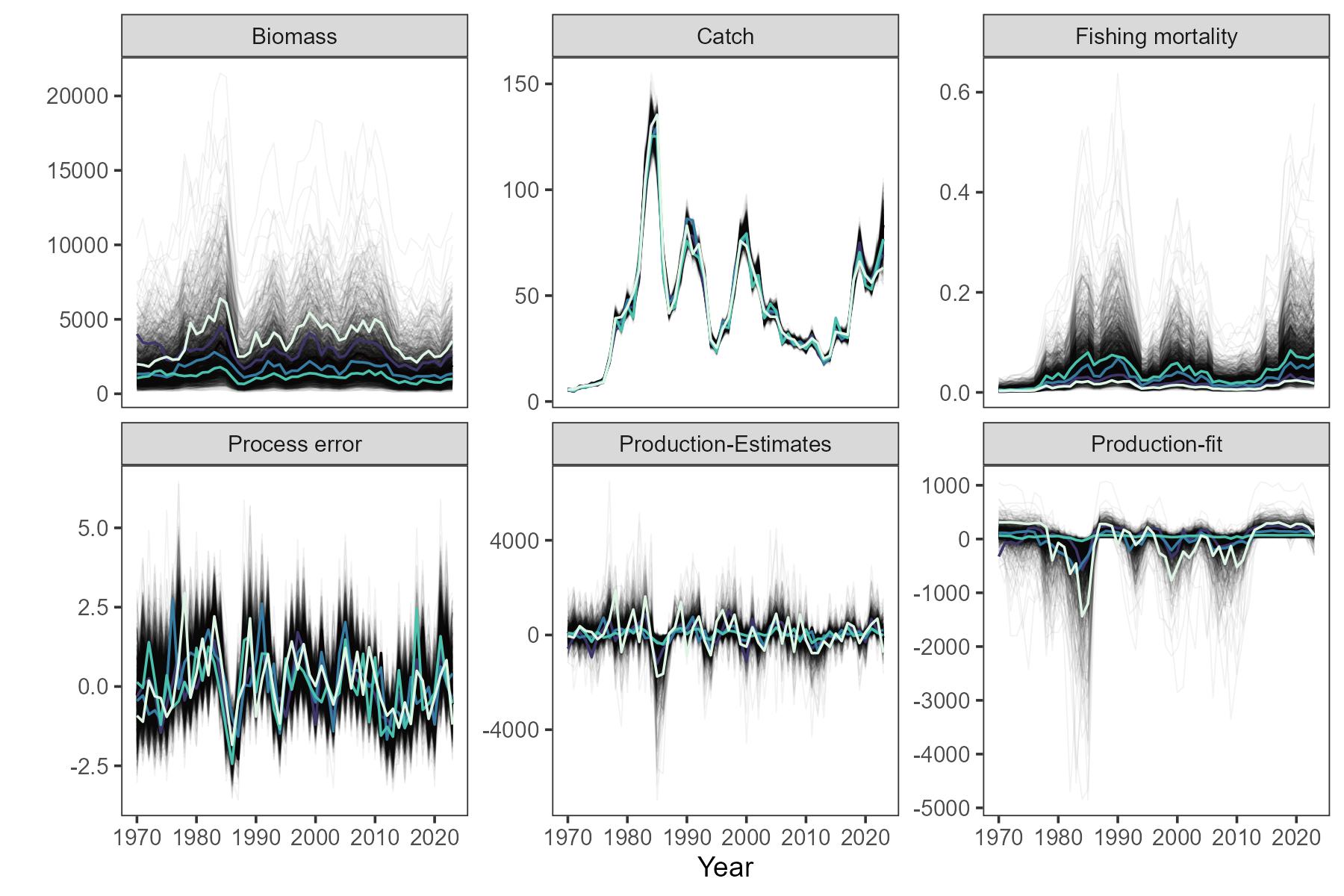
The simulation model of future process errors used a random normal distribution with parameters equal to the sample mean and standard deviation of the estimated annual process errors. As with the fixed effect parameters, each iteration of the MSE was based on stochastically drawn mean and standard deviation for the random normal process errors. Example simulated distributions of the process errors and the corresponding trajectories of biomass and catch over the historical period are shown in Figure 5.

Alternative models for the simulation of process noise were explored. A first-order autoregressive model produced similar annual variability as the simple normal model, while a random walk model resulted in unrealistically high biomass compared to historical SPiCT estimates. Consequently, the aproach using random normal errors was retained.

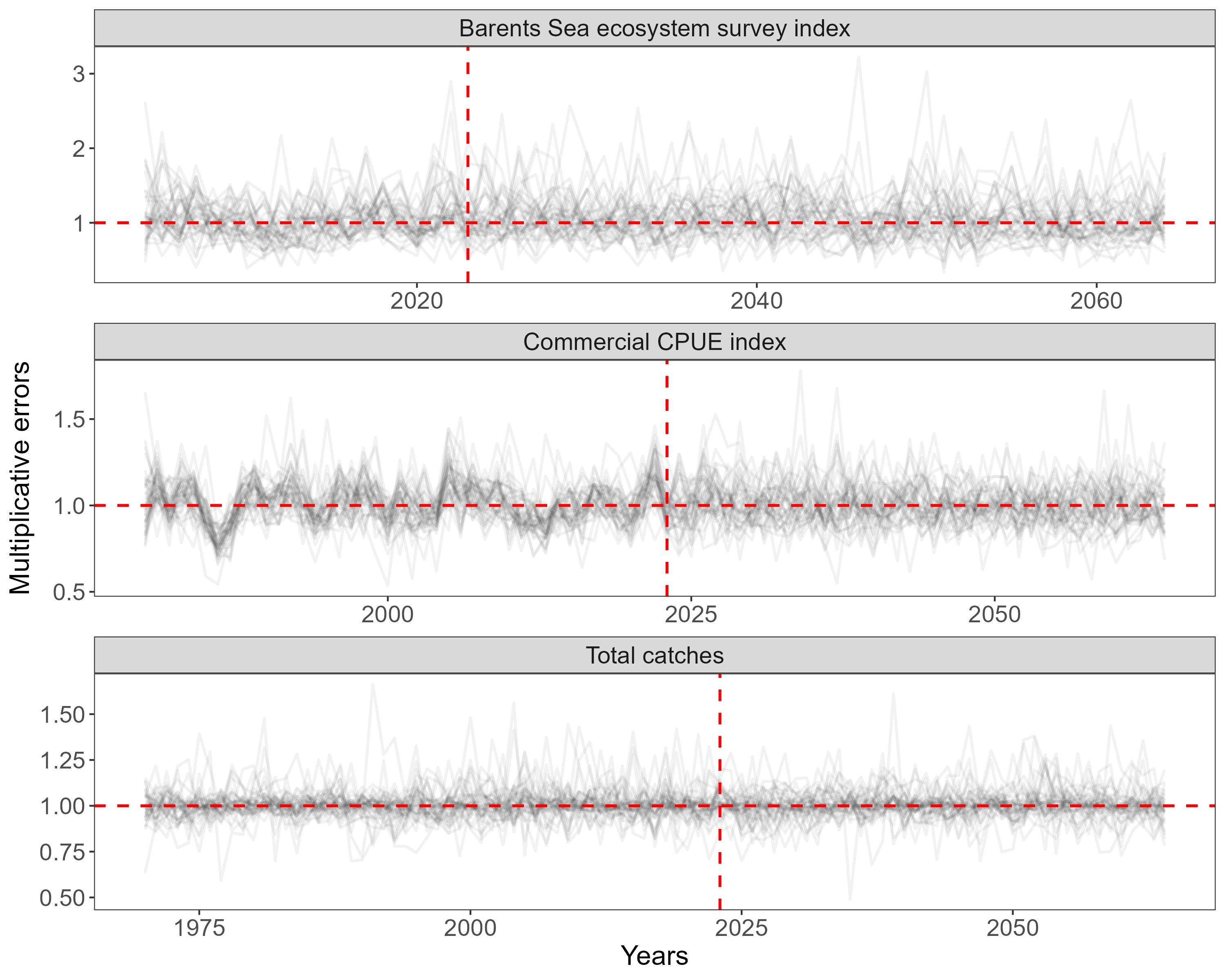
2.3 - Observation model

Survey and CPUE indices were computed in log-space as the product of a scalar (q) and ‘true’ biomass from the OM with additional simulated random normal error. SPiCT allows user specification of sub-annual timing for stock indices (as a fraction of the year), therefore the index parameter estimates from SPiCT cannot be directly applied to our observation model that operates on annual time-steps. As a workaround, survey-specific q and its standard deviation were recalculated by computing the log-mean and standard deviation of the differences between the log of the observed index values and log of the SPiCT estimated biomass at the start of each year. Assuming the same biomass index equation used in SPiCT (log I =log q/B +ϵ), the log-mean of the residuals described in the previous sentence is the new log q. This equation can be rewritten as log I =log q +log B, then log q =log I -log B. The standard deviation of these residuals is the standard deviation of the ‘new’ observation error. This simplification implicitly incorporates the sub-annual production and process error from SPiCT into these new q values and their uncertainty. Annual observation errors are assumed independent random draws from the estimated normal distribution. Example simulations to illustrate the generated errors are shown in Figure 6.

Only two of the four survey indices, the biomass index from the Barents Sea ecosystem survey (BESS), and the commercial CPUE index, were generated from the observation model as these are the only indices based on ongoing data collection (two indices are based on historic surveys that have been replaced by the BESS). Indices of the projected biomass are then fed into the estimation model within the MSE simulation loop.

2.4 - Implementation model

No implementation error is accounted for in the MSE. The realized catch in the OM will match the TAC from the decision model if the ‘true’ biomass exceeds the TAC. Historically, the shrimp fishery has operated de facto as an open-access fishery, but with catches corresponding to estimated F values far below the most recent estimated F_MSY (IMR-PINRO 2023). This is likely because of shrimp prices and fuel costs as limiting factors, resulting in a fishing mortality that optimize net revenues for the fishery below the estimated F_MSY (Lancker 2023). This current understanding has informative implications for perfect implementation of the proposed HCR using F_MSY and B_MSY as control parameters; realized fishing will likely remain below the advised F_target from the proposed HCR under current price and cost constraints. If any of the proposed HCR is precautionary according to the ICES risk criterion (<5% risk of falling below B_lim), any other implementation scenario attempting to emulate historical fishing behavior with lower F than F_target will be even less risky and can, thus, be assumed to be precautionary. Furthermore, assuming no mismatch between the advice and realized catch in the MSE avoids arbitrary and potentially misleading scenarios for management performance under future fishing, as well as the difficulties of configuring models for scenarios that do not implement the HCR but include other, extrinsic (e.g. economic) dynamics. However, the configuration of the implementation model should be revisited in the future based on an improved understanding of past or present fleet dynamics or if F in the fishery is close to or exceeds F_MSY.

2.5 - Management procedure

2.5.1 - Estimation model

The assessment model (SPiCT) was used as the estimation model, with the same model configurations and data inputs. The data inputs were updated in every projection year with the simulated stock indices and total catch. For running the short-term forecast (STF), the same settings as in the assessment and the built-in functions within the spict R package were used.

The sequence of computations in the estimation model, STF and TAC implementation were as follows:

1. The estimation model estimated biomass at the start of year y using data inputs up through year y-1.

2. The STF projected the biomass at the start of year y forward to year y+1 using the target F output from the HCR. There is currently no lag in management as the annual stock assessment is conducted at the end of the year ahead of the new TAC year of the shrimp fishery. Surplus production was also projected in year y. The catch corresponding advised F was used as the TAC for year y.

3. The TAC from the STF was translated to ‘realized’ catch in the implementation model.

The estimation model outlined above is typical of a ‘full-loop’ MSE (ICES 2019a). However, additional modifications had to be made to the estimation model in order to allow the SPiCT model to converge in a majority of the MSE simulations. These modifications are further detailed in the section "2.9 Tailored configuration for the shrimp MSE".

2.5.2 - Candidate management strategies in the decision model

The decision model comprises both the HCR, TAC computation, and any subsequent modification of the TAC. The candidate HCR’s proposed for the Barents Sea shrimp are illustrated in Figure 1.

Ftarget and B_trigger are control parameters in the HCRs, and B_lim is the reference point defining the general biomass level below which production becomes compromised. The control parameters and B_lim are determined by the MSY reference points (F_MSY and B_MSY) estimated by SPiCT every year. Ftarget is set to the F_MSY or a fraction thereof, B_trigger is set to 0.5 * B_MSY, and B_lim is approximated by 0.3 * B_MSY (IMR-PINRO 2023).

A stability mechanism for catches is included with all HCR options in the form of a TAC constraint. The constraints proposed are that TAC may not be more than 20% above (i.e. TAC(y+1) <= 1.2 TAC(y) ) or 20% below (i.e. TAC(y+1) >= 0.8 TAC(y)) the previous TAC.

2.6 - Alternative operating model: Shift in carrying capacity (OM2)

Northern shrimp stocks have been observed to vary substantially (Hvingel 2021). These dynamics are to some extent attributed to changes in the stock production, likely driven by environmental changes and/or changes in predation pressure. Historically, the Barents Sea stock has been relatively stable, but evidence from other shrimp stocks suggests that low production periods may also occur in the Barents sea. The Flemish Cap stock, for instance, showed large fluctuations linked to variation in predator stocks (Pérez-Rodríguez 2012), and the West Greenland shrimp stock experienced a doubling in catches when it shifted from a period of high to one of low predation intensity (Hvingel 2006). The West Greenland stock is comparable in size to the one in the Barents Sea and has shown similar resilience to environmental changes (in contrast to the Pacific stock and the North Atlantic stocks further south). While an increase in productivity could promote greater yield, a sudden drop in productivity can increase the risk of overfishing and is therefore a management concern. To simulate such a drop in productivity, OM2 therefore assumed a reduction in the current estimated carrying capacity (K) by half midway through the projection period of MSE simulations. The large assumed decrease in K ensures OM2 represents a robustness scenario to test the set of precautionary HCRs under OM1.

2.7 - Number of replicates and projection years

The number of replicates or iterations in a MSE is an important consideration for the computation of risk as defined by ICES, which relies on the tails of the simulated biomass distribution from the MSE (ICES 2019a). We simulated 2000 iterations where each iteration varied the starting biomass, set of parameters, and time series of future process and observation errors. Generally, 2000 iteration were considered adequate in other MSE (ICES 2019a) when using the risk3 definition for the precautionary criterion (ICES 2022, ICES 2019a). HCR performance can be sensitive to the specific risk definition (Thorpe and De Oliveira 2019), but here we followed standard ICES procedures and did not explore the risk sensitivity.

A projection period of 40 years is used in the MSE so that management performance may be evaluated over a sufficiently long term, while being similar to the projection times of previous MSE for other stocks (ICES 2019a, ICES 2019b, ICES 2024).

2.8 - Performance statistics

The performance statistics directly represent the metrics listed in the request. Specifically, the short-term is interpreted as 2025-2029, medium-term is 2030-2039, and long-term is 2040-2064. For the values of biomass relative to B_MSY, yield relative to MSY, and fishing mortality relative to F_MSY, each are first calculated for each iteration and year (where there are unique B_MSY, MSY, and F_MSY values for each iteration), then the median taken across years within each respective term (short-, medium-, and long-term) for each iteration, and then the median of these values across iterations within each term. For the probability of biomass falling below B_lim, we use the risk3 definition from ICES workshop on guidelines for MSE (ICES 2019a), which involves two computational steps: 1) calculate the proportion of iterations where biomass is less than B_lim for each year (where B_lim is defined as 0.3 B_MSY) then 2) take the maximum proportion across years. A probability (risk3) is calculated for the short-, medium-, and long-terms. The probability of the biomass falling below B_trigger (0.5 B_MSY) is calculated in the same manner. Finally, the average percent quota change is computed as the mean of the absolute value of the relative differences in the TAC (i.e. divided by the previous year’s TAC), first taken over the years within a specific term and then over iterations.

2.9 - Tailored configurations for the shrimp MSE

During the setup and initial projections of the shrimp MSE, a high number of MSE iterations were encountered where the estimation model did not converge in at least one projection year. Upon further investigation, it became evident that the large range of population biomasses used at the start of the projection period in the operating model resulted in observations that the SPiCT model had difficulties fitting. This was largely due to informative priors on the carrying capacity (K) and starting depletion level (B/K). By using less informative priors in the estimation model, the convergence rate across iterations and years improved.

Instances of non-convergence persisted, however, necessitating further adjustments. Per the spict package guidelines, non-convergence can be addressed by shortening the catch time series to match the time span of the survey biomass indices. Implementing this option on its own improved SPiCT convergence across iterations, but did not entirely resolve the issue. Thus, a semi-iterative model-fitting approach was implemented in the estimation model to sequentially check SPiCT non-convergence, modify input, and refit until convergence occurs. The implemented procedure emulated, therefore, a (limited) model tuning approach, as commonly applied in reality, increasing the ‘realism’ of the estimation model. This iterative procedure resulted in most estimation models converging across MSE iterations and years. The code for this semi-iterative procedure is shown in the Annex.

The third issue regards the treatment of zero catch observations within the SPiCT model. The fit.spict function from the spict package removes zero catch observations before model fitting, and treats them as missing where SPiCT still estimates fishing in these zero catch years. This proved problematic in MSE simulations because some of the proposed HCRs will output F = 0 when estimated B<B_lim resulting in zero TAC and subsequently zero catch observations. The estimation of fishing by SPiCT when it is known that no fishing occurred induces otherwise avoidable bias in the estimation model and produces incorrect advice. This SPiCT behavior is not easily resolvable within the base code. A quick workaround was implemented in the MSE by setting F to a very low value (e.g. 0.01) instead of B_lim in the decision model to produce catches in all years. The biggest caveat is that this modification creates HCRs that are not the proposed HCRs, although in a realistic setting it can be expected that even under a closed fishery the shrimp stock would experience some minor fishing mortality (from scientific surveys, by-catch in other trawl fisheries, etc). The resulting very low catches had minor impacts on performance metrics, and even less so on ranking of the HCRs.

3.1 - HCR performance against OM1

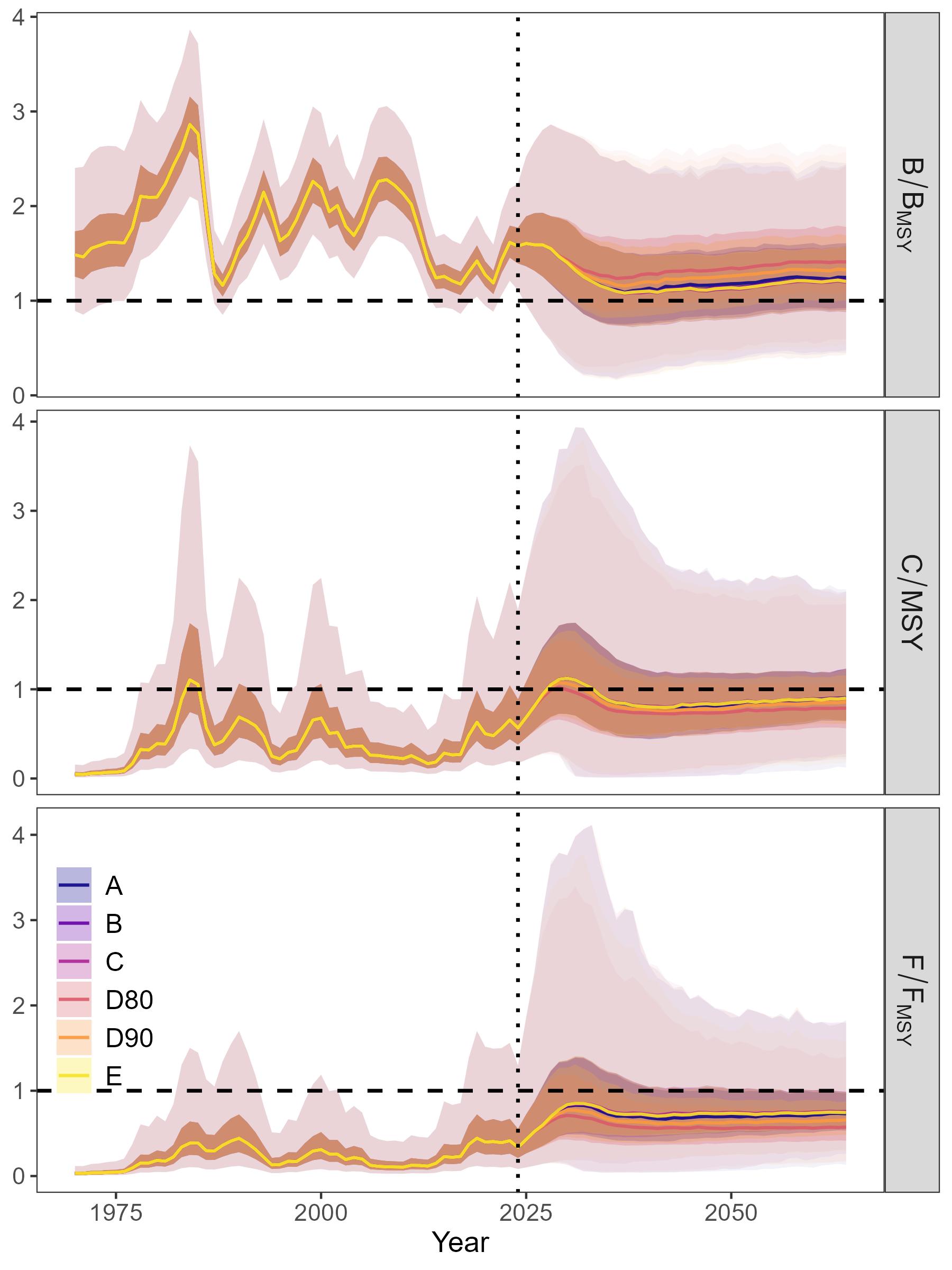
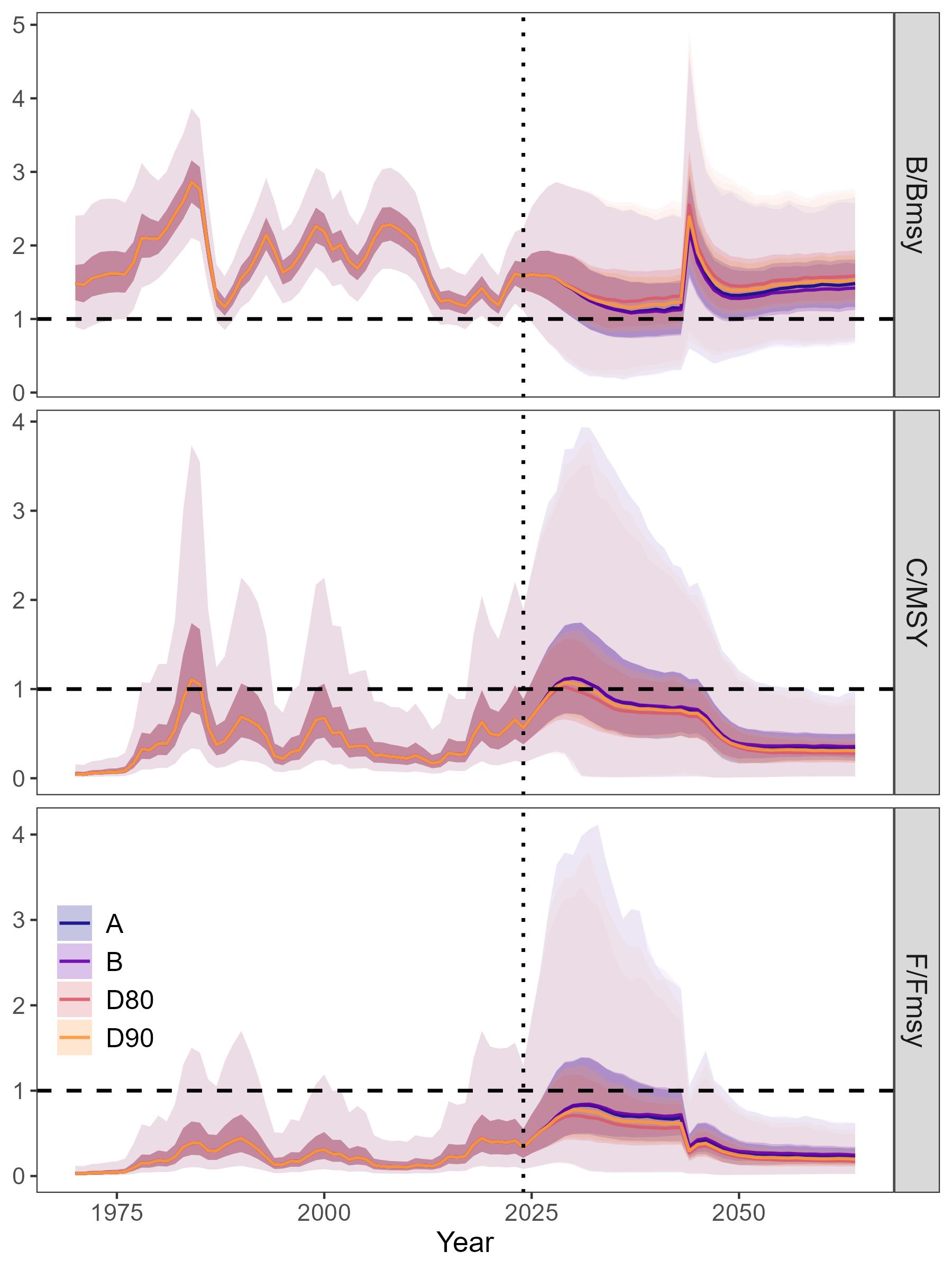
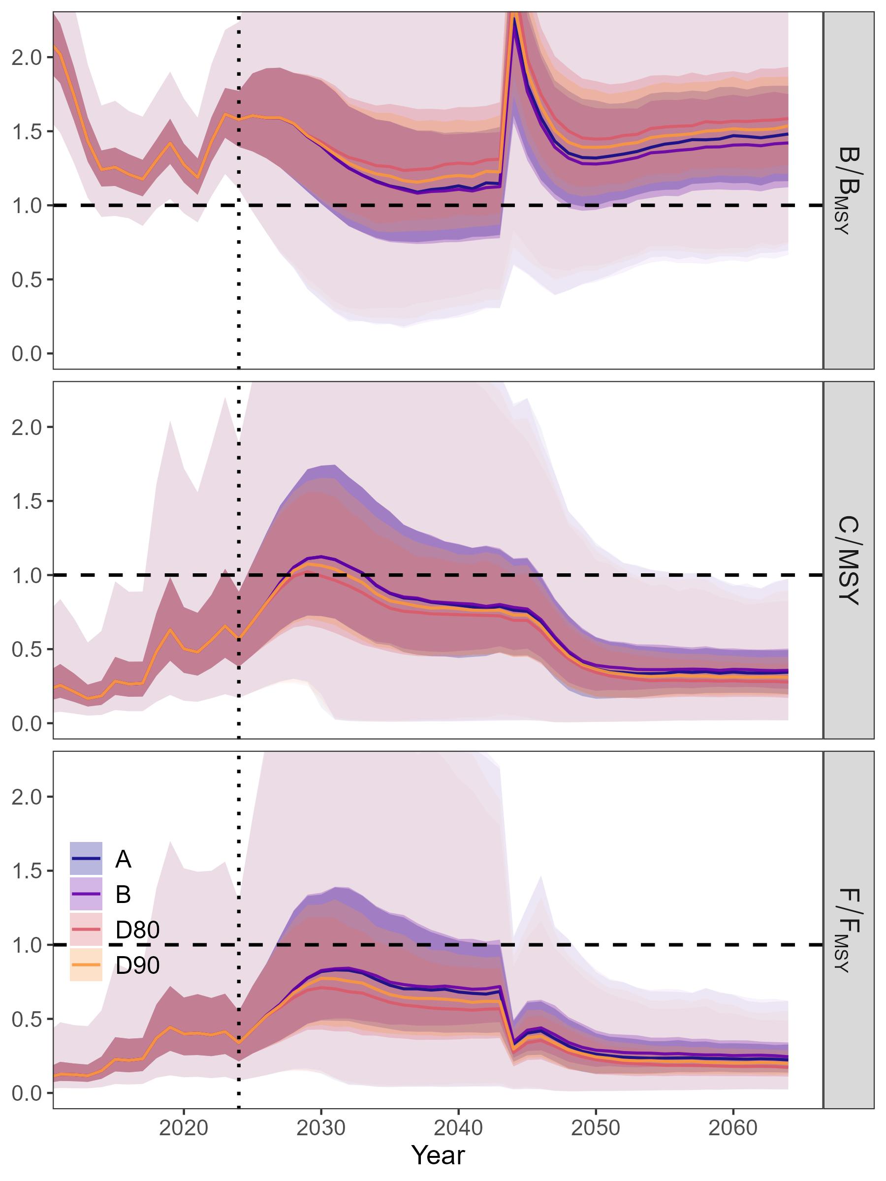
Under OM1, all HCRs showed similar relative biomass and catch trajectories with wide uncertainty (Figures 7 and 14). All HCRs resulted in biomass decline during the first ten years, as most starting biomass (in 2024) was at or above B_MSY and fishing ramped up to F_target (equal to or less than F_MSY, depending on the HCR). Fishing stabilized in the long-term, while biomass slowly and continuously increased. No HCRs caused average F to exceed F_MSY. Similarly, average biomass remained above B_MSY under all HCRs. HCRs D80 and D90 differed most from the other trajectories, maintaining the highest average biomass, but lowest average yield.

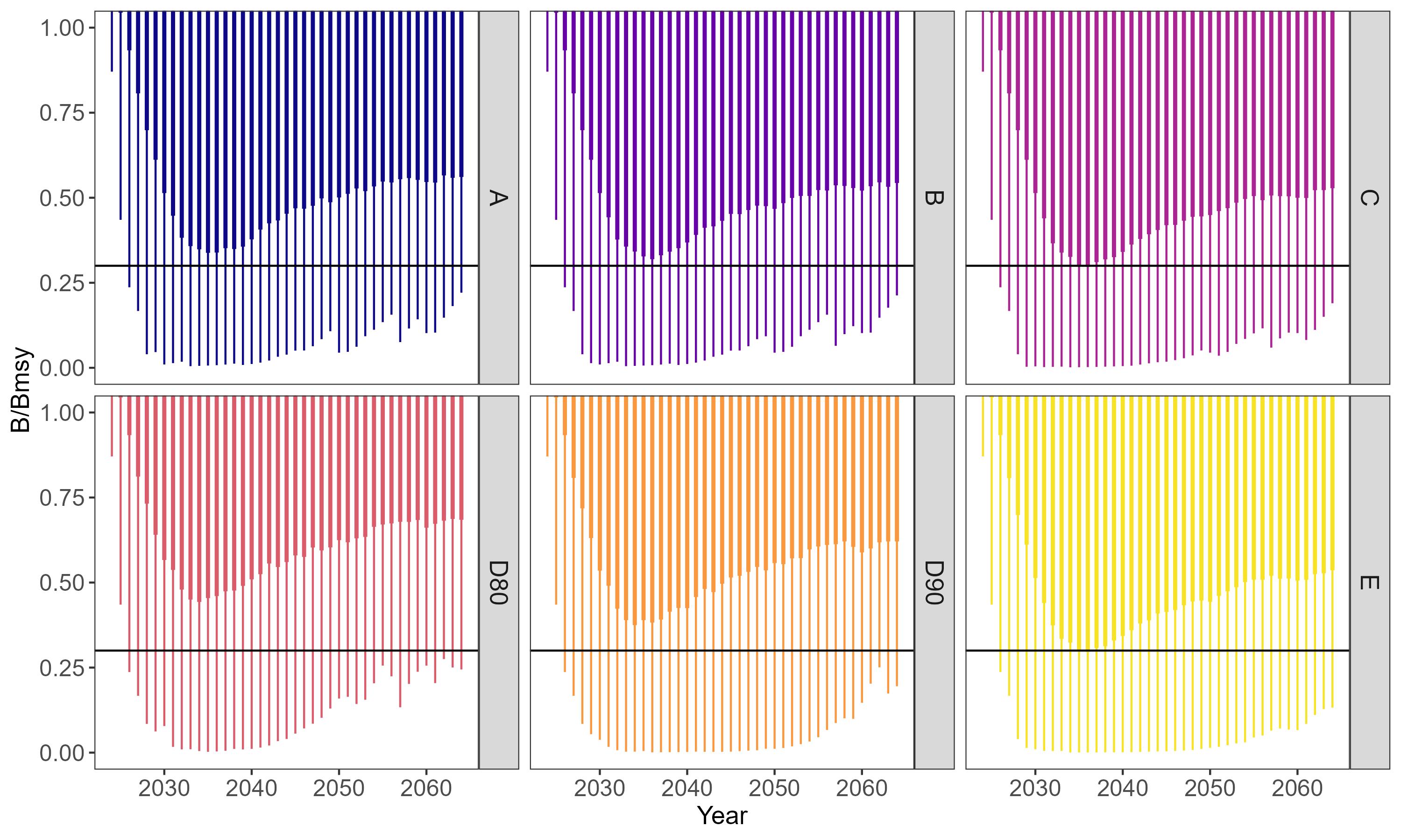
The annual risk of each HCR causing the stock to drop below B_lim was similar across HCRs (Figure 8). In general, the greatest risk occured in the short-term, when fishing ramps up in accordance with each HCR starting from biomass well above each HCR’s B_trigger.

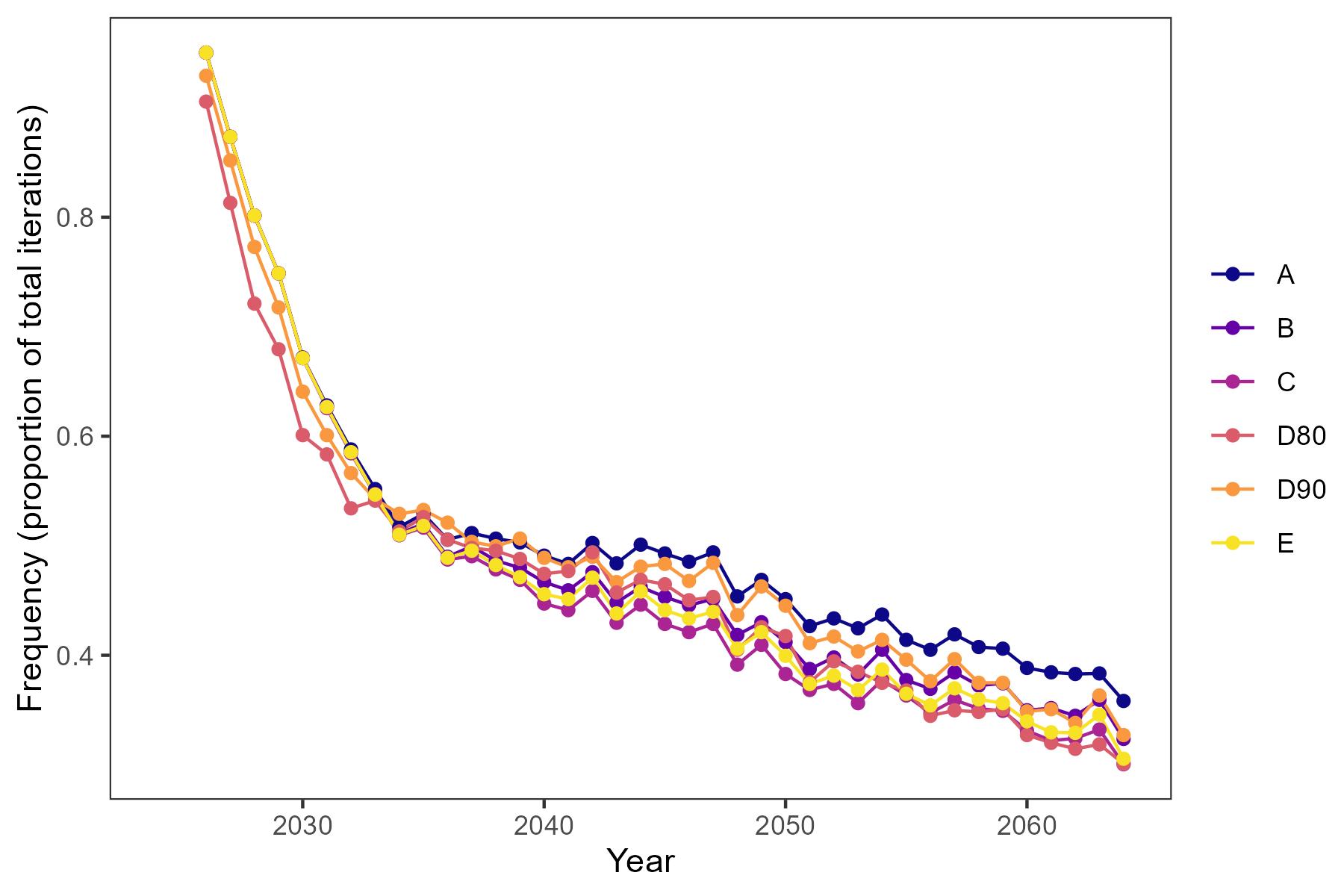
The TAC stability mechanism of +/-20% was frequently triggered at the start of the projection period, but then the frequency rapidly dropped in the short-term, and continued to gradually decline in the long-term (Figure 9). Importantly, without the mechanism, fishing in the short-term would increase more rapidly, likely increasing the risk of stock collapse. The frequencies for each HCR are similar (e.g. within approximately 0.10 of each other), although HCR A triggered the TAC constraint most frequently in the long term.

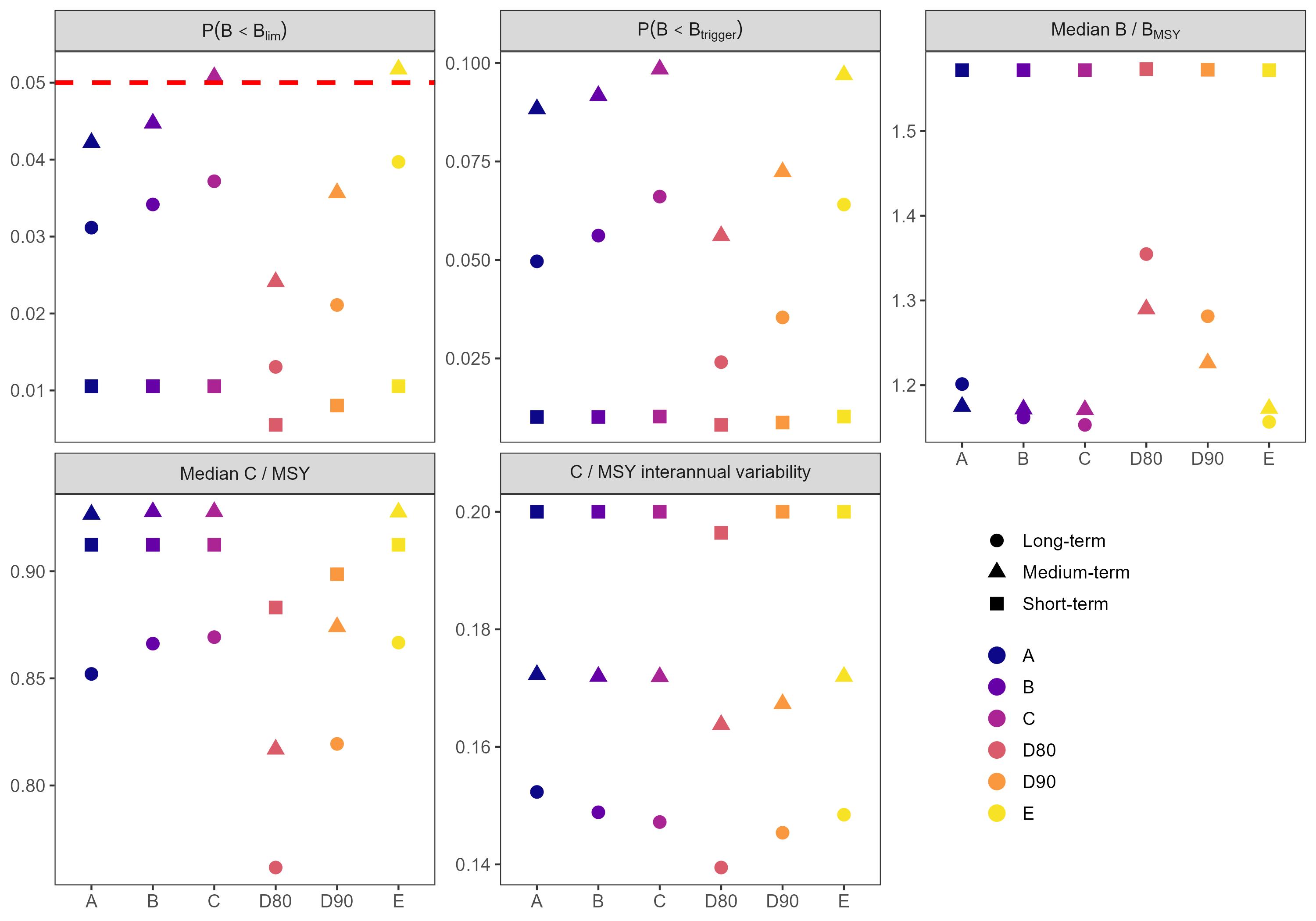
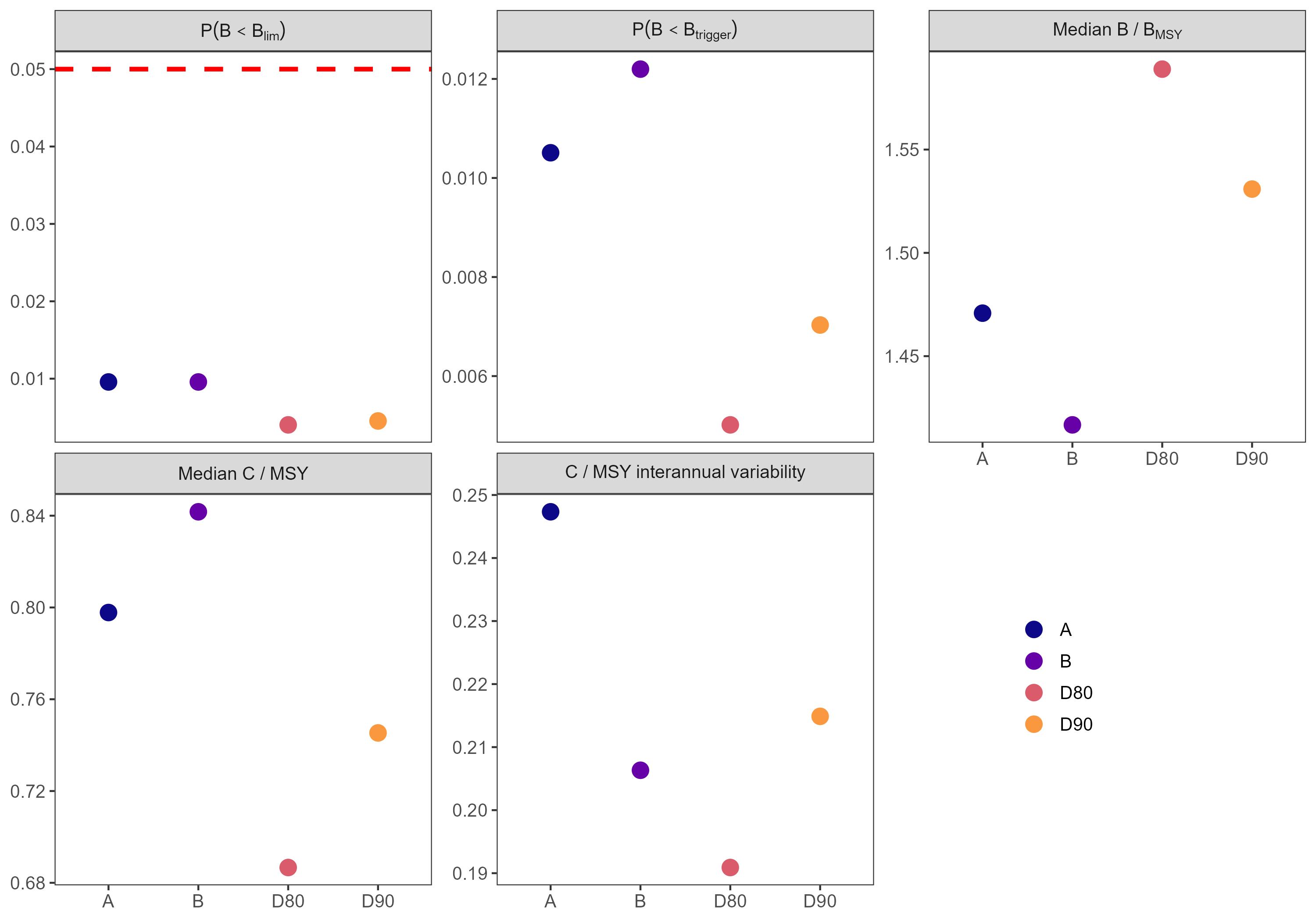
The performance metrics for the pre-specified time periods were similar across all HCRs with some key differences (Figure 10). First, HCRs C and E caused a risk (i.e. P(B<B_lim)) greater than 0.05 in the medium-term, violating the criterion for precautionarity. HCRs that are not precautionary should not be further considered by management, and thus we focused on comparing the remaining precautionary HCRs. In general, all HCRs showed the highest relative biomass and catch in the short-term, reflecting the median starting point of the simulations at biomass above B_MSY. Both biomass and catch stabilized at lower levels in the longer term, as a result of the HCRs. All precautionary HCRs maintained average biomass above B_MSY and average catches relatively close to MSY (e.g. within 0.75 of C/MSY) in all periods.

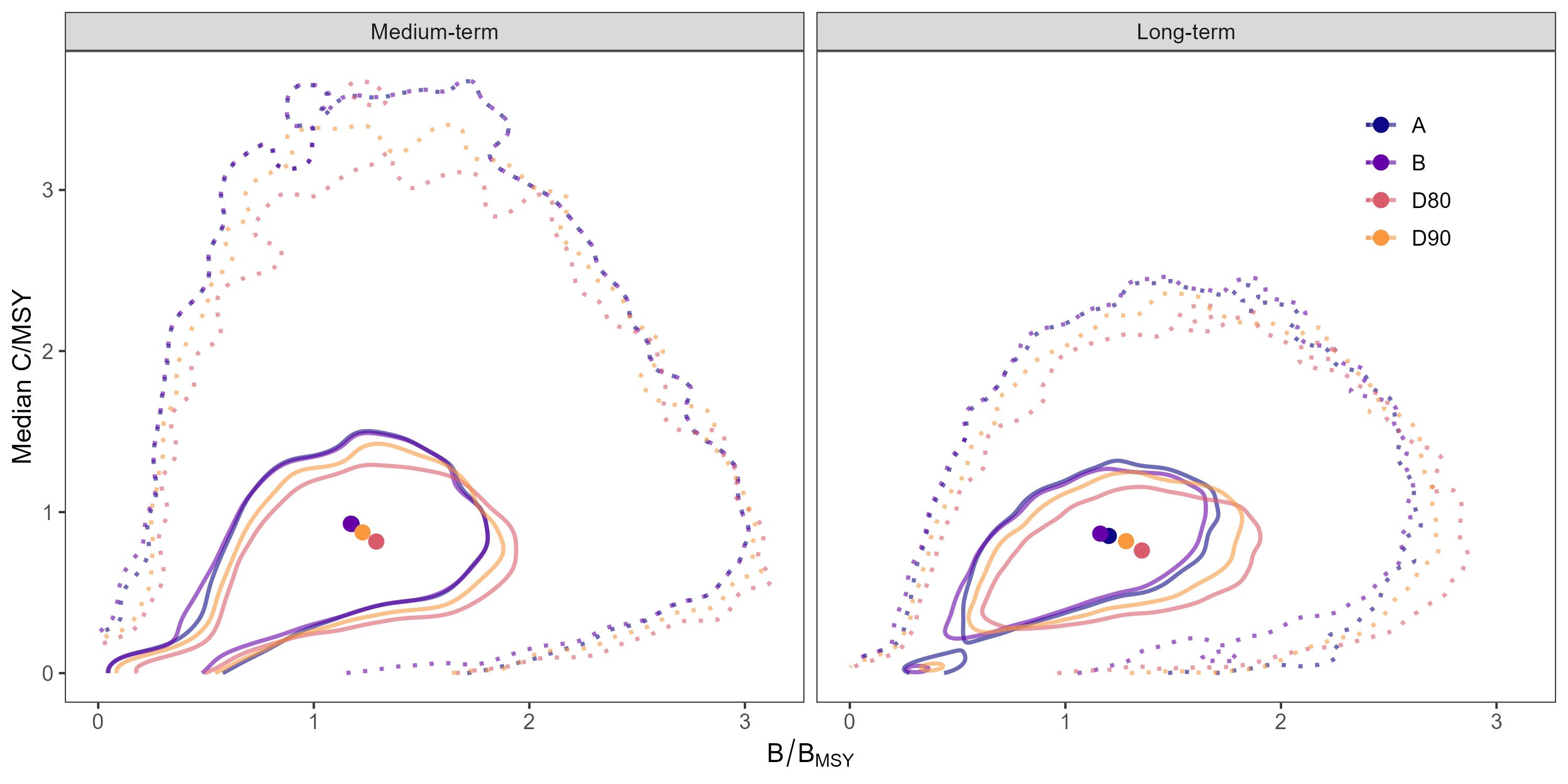
Between the precautionary HCRs, the main differences were caused by the definition of F_target. HCRs A and B with F_target = F_MSY resulted in higher median catches, but also higher risk, lower biomass and slightly higher catch variability compared to HCRs D80 and D90 with F_target < F_MSY. The latter were generally more precautionary, trading off less risk and higher biomass levels with lower median catches. This contrast in performance was most pronounced between HCRs B and D80, although the differences between A and B were very marginal. The differences between D80 and D90 were larger, with D80 producing the lowest catches while allowing the highest relative biomass in the long-term, lowest catch variability, and lowest recurrence of biomass falling below B_trigger (i.e. low P(B<B_trigger)). While HCRs D80 and D90 may appear to show greater relative contrast from HCRs A and B, when accounting for between-iteration variability in median relative biomass and catch, the resulting distributions mostly overlap (Figure 11).

3.2 - HCR performance against OM2

While a reduction in the carrying capacity reduced the absolute biomass immediately after occurring due to reduced production, the relative biomass (B/B_MSY) showed an increase because the reduced carrying capacity also reduced the B_MSY reference point (Figure 12 and 15). Importantly, all HCRs caused a prompt reduction in fishing and relative catches, largely due to the estimation model being able to quickly adjust biomass estimates (even without explicit incorporation of a shift in carrying capacity).

The HCRs that were precautionary under OM1 remained precautionary under OM2. However, during the period after the reduction in carrying capacity, more contrast was found between the HCR performance compared to the performance under OM1 (Figure 13). Notably, HCR A showed the highest catch variability, but was similar to HCR B in terms of probability of decreasing below B_trigger (where HCR A < HCR B), median relative biomass (where HCR A > HCR B), and median relative catch (where HCR A < HCR B). As under OM1, HCRs D80 and D90 remained more conservative than HCRs A and B, with very low probability of biomass falling below B_trigger and higher relative biomass, but lower relative catch compared to HCRs A and B (with biomass from HCR D80 > HCR D90, and catch from HCR D80 < HCR D90). A noteworthy difference compared to OM1 was a higher catch variability of D90 under OM2 compared to B.

3.3 - Extreme stock conditions

The wide uncertainty in starting absolute biomass projected from 2024 resulted in few iterations with absolute biomass levels that were lower than the TAC produced from the HCRs. To prevent the stock from going negative (which is computationally problematic), fishing was still simulated in these instances, but at the previous year’s fishing mortality instead of the advised TAC. Because this may not reflect the true management response in such cases, these iterations were removed from the following performance metrics and projections calculated below. Under OM1, 10 of 2000 iterations were removed, or 0.5% of all simulations. As a check, we computed the performance metrics with all 2000 iterations and there was no difference in the comparative performance of the HCRs and precautionary determinations (not shown).

Out of six HCR evaluated, the four without any fishing at biomass levels below B_lim were found to be precautionary. Of these precautionary HCRs, all performed similarly in simulations and thus may be viable HCRs for management to implement. Contrasts in performance were mostly linked to the definition of F_target, with the HCRs D80 and D90 being more risk-averse as a result of using a F_target at 80% and 90% of F_MSY, respectively. A key management decision is therefore between HCRs D80 and D90 vs A and B, weighing less risk, higher median stock biomass and less catch variability against lower catches relative to MSY on average for D80 and D90 compared to A and B. The median catches of D80 and, to a lesser degree, D90 may be considered undesirably low at less than 80% of MSY, especially under OM2. However, they represent still a significant increase compared to current total catches that have been at less than 50% of MSY for most of the past two decades.

There is substantial uncertainty linked to the simulated increase of catches from the current fishing mortality to a F_target at or near F_MSY, and many differences between the HCRs can be considered negligible in this context. This applies in particular on differences between HCRs A and B that were very marginal. From a practical standpoint, however, the vertical cutoff of fishing at B_lim (fishing drops immediately to zero from that equal to 0.5*F_MSY) may be undesirable for the fishery stability, even though it has the benefit of decreasing TACs more slowly when biomass is below B_trigger and simulations did not show a substantial effect of the cutoff (e.g. in terms of higher catch variability). Furthermore, any scenario where future total catches remain for economic or other reasons below the adviced TAC based on any of the four precautionary HCRs can be considered precautionary as well.

4.1 - Recommendations

A subset of candidate HCRs performed well, including under an alternative scenario of decreased productivity, and can therefore be considered robust. However, to improve on the current results and address main sources of uncertainty, it was recommended to explore the following points in future MSE analyses and research:

• Uncertainty from the stock assessment propagates into the MSE as wide distributions of starting values. Higher fishing mortality based on the HCRs may help to improve stock estimates by providing the assessment model more information about how the stock responds to higher fishing pressure and, thus, its productivity. Fine-tuning and integration of additional data into the assessment model as previously recommended (Hvingel and Zimmermann 2024) may also contribute to reduced uncertainty. An updated MSE and re-evaluation of HCRs is therefore recommended after fishing mortality has been at higher levels for several years.

• As an important forage species in the Barents Sea, northern shrimp is subject to bottom-up and top-down pressures from the environment and predation, respectively. The MSE has accounted indirectly for many of these environmental-ecological dynamics by including uncertainty between iterations (both process and observation errors), and by testing an alternative scenario of drastically reduced carrying capacity. Thus, the evaluated HCRs can be considered robust against impacts of environmental change or ecosystem dynamics. The MSE showed, furthermore, the capability to detect and account for large shifts in stock productivity with the current assessment framework. Nevertheless, potentially positive effects of the current large decrease in the Northeast Arctic cod stock, a major shrimp predator, and the expected negative impacts of climate change (Kjesbu 2022) should be investigated and quantified, with the goal to explore these dynamics more explicitly in a future MSE. Considering the important predator-prey link of cod and shrimp, future MSEs and management strategies should ideally include explicit species interactions in a multi-species framework.

• The MSE focused solely on biological dynamics and performance, ignoring the real-world fleet dynamics and economic constraints of the fishery that may likely prevent a sudden increase of fishing effort to levels needed to achieve F_target of the HCRs. From a management perspective, this is not problematic as logic dictates that any level of fishing below F_target (i.e. the underfishing of advice based on the evaluated HCRs) remains precautionary. However, considering the characteristics of the fishery, it is recommended to investigate the fleet dynamics further and expand the current MSE framework with bioeconomic components that allow for a more realistic simulation of the fishery. The incorporation of economic reference points and targets such as maximum economic yield should be considered in a future MSE.

Berg, C., Coleman, P., Cooper, A., Hansen, H. Ø., Haslob, H., Herrariz, I. G., Kokkalis, A. 2021. Benchmark Workshop on the development of MSY advice for category 3 stocks using Surplus Production Model in Continuous Time; SPiCT (WKMSYSPiCT).

Fletcher, R. 1978. Time-dependent solutions and efficient parameters for stock-production models. Fish. Bull, 76: 377–388.

Hvingel, C. 2006. Construction of biological advice for the management of a northern shrimp fishery–the West Greenland example. UITØ, Norges Fiskerihøgskole.

Hvingel, C., Sainte-Marie, B., and Kruse, G. H. 2021. Cold-water shellfish as harvestable resources and important ecosystem players. ICES Journal of Marine Science, 78: 479–490. 10.1093/icesjms/fsab005.

Hvingel, C., and Zimmermann, F. 2024. Barents Sea Shrimp - stock assessment report 2023. Report. https://www.hi.no/hi/nettrapporter/imr-pinro-en-2023-11.

ICES. 2019a. Workshop on Guidelines for Management Strategy Evaluations (WKGMSE2). Report. ICES Scientific Reports. 10.17895/ices.pub.5531.

ICES. 2019b. Workshop on North Sea Stocks Management Strategy Evaluation (WKNSMSE). Report. ICES Scientific Reports. 10.17895/ices.pub.5090.

ICES. 2022. Report of the Workshop on Guidelines for Management Strategy Evaluations (WKGMSE). Report. ICES Expert Group reports (until 2018). 10.17895/ices.pub.5304.

ICES. 2024. Workshop on a long-term management strategy evaluation for the Northern shrimp (Pandalus borealis) in divisions 3.a and 4.a East (Skagerrak and Kattegat and northern North Sea in the Norwegian Deep) (WKPANDLTMSE). Report. ICES Scientific Reports. 10.17895/ices.pub.22434577.v1.

IMR-PINRO. 2023. Advice on fishing opportunities for Barents Sea shrimp in 2024. Report. https://www.hi.no/hi/nettrapporter/imr-pinro-2023-12.

Kell, L. T., Mosqueira, I., Grosjean, P., Fromentin, J.-M., Garcia, D., Hillary, R., Jardim, E. 2007. FLR: an open-source framework for the evaluation and development of management strategies. ICES Journal of Marine Science, 64: 640–646.

Kjesbu, O. S., Sundby, S., Sandø, A. B., Alix, M., Hjøllo, S. S., Tiedemann, M., Skern-Mauritzen, M. 2022. Highly mixed impacts of near-future climate change on stock productivity proxies in the North East Atlantic. Fish and Fisheries, 23: 601–615. https://doi.org/10.1111/faf.12635.

Lancker, K., Voss, R., Zimmermann, F., and Quaas, M. F. 2023. Using the best of two worlds: A bio-economic stock assessment (BESA) method using catch and price data. Fish and Fisheries. https://doi.org/10.1111/faf.12759.

Pedersen, M. W., and Berg, C. W. 2017. A stochastic surplus production model in continuous time. Fish and Fisheries, 18: 226–243. https://doi.org/10.1111/faf.12174.

Pella, J. J., and Tomlinson, P. K. 1969. A generalized stock production model. Inter-American Tropical Tuna Commission, Bulletin, 13: 419–496.

Pérez-Rodríguez, A., Koen-Alonso, M., and Saborido-Rey, F. 2012. Changes and trends in the demersal fish community of the Flemish Cap, Northwest Atlantic, in the period 1988–2008. ICES Journal of Marine Science, 69: 902–912. 10.1093/icesjms/fss019.

Punt, A. E., Butterworth, D. S., Moor, C. L. de, De Oliveira, J. A. A., and Haddon, M. 2016. Management strategy evaluation: Best practices. Fish and Fisheries, 17: 303–334. doi:10.1111/faf.12104.

Thorpe, R. B., and De Oliveira, J. A. A. 2019. Comparing conceptual frameworks for a fish community MSY (FCMSY) using management strategy evaluation—an example from the North Sea. ICES Journal of Marine Science, 76: 813–823. 10.1093/icesjms/fsz015.

6.1 - Estimation model tuning

Code that was used to implement conditional model-tuning for the estimation model to handle failed convergence:

# Fit spict with default / standard model setting
fit <- fit.spict (input,...) convd <- 0 if (fit $ opt $ convergence == 0 & all ( is.finite (fit $ sd))){
# If model has converged, set an integer code indicating convergence occurred on first try
convd <- 1 } else { # If non-convergence, set weaker priors
input$priors$logK <- c ( 7.4 , 1.4 , 1 ) # Carrying capacity
input$priors$logbkfrac <- c ( log ( 0.75 ), 0.5 , 1 ) # Initial depletion
# Re-fit
fit <- fit.spict(input,...)
if(fit$opt$convergence == 0 & all ( is.finite (fit$sd))){
# If model has converged, set an integer code indicating
# convergence occurred on second try (weaker priors)
convd <- 2 } else { # If STILL non-convergence, shorten catch time frame
input <- shorten.inp(input, mintime= 1980)
# Re-fit
fit <- fit.spict (input,...)
if(fit$opt$convergence == 0 & all ( is.finite (fit $ sd))){
# If model has converged, set an integer code indicating
# convergence occurred on third try (shortened catches)
convd <- 3 } } }

6.2 - Simulation trajectories

6.3 - Reviewer reports

Reviewed by: J.Jonasson, HAFRO, Iceland.

The reviewer wants first to commend the authors and their team for a great and thorough management strategy evaluation on the northern shrimp (Pandalus borealis) stock in the Barents Sea (ICES subareas 1 and 2). Six candidate HCRs were tested, based on agreement from stakeholders on the 29th of August 2023, between the Institute of Marine Research, Directorate of Fisheries, and industry representatives from Fiskarlaget, Fiskebåt, Sjømat Norge and Norges Råfisklag. The four candidate HCRs that halted fishing when Blim was reached surpassed the precautionary criteria of less than 5% risk of falling below limit reference point for spawning stock biomass, B_lim. In the history of the assessment, now carried out with the assessment model SPiCT, the estimated F values are far below the most recent estimated F_MSY and it has operated in fact as an open access fishery, as discussed in the report. This is not an ideal situation for MSE evaluation, but as talked about, it warrants that future work should include or explore external or economic dynamics as well.

The report also analysed an alternative scenario (OM2), were there was an abrupt shift in carrying capacity, as can occur through change in productivity or increase in predation. This in an important addition to the MSE for a sensitive species like the northern shrimp. All the four candidate HCRs performed well under the OM2 scenario and the more conservative HCRs of D80 and D90, had lower probability of biomass falling below B_trigger and maintained higher relative biomass. The relative catches for HCRs A and B are of course higher then for HCRs D80 and D90, but the latter are expected to maintain higher biomass and in most cases lesser variability in catches, which is closer to historical fishing pattern. Impressingly, the estimation model quickly adjusted the biomass estimates, and all HCRs caused a sharp reducion in harvest under the changing scenario.

Recommendation put forward look unerring and touch upon important issues. Adopting more complicated model that would include predation of species like the Atlantic cod in the estimation model might help to explore and understand the dynamics of the stock better. However, as shown in this work, current model and proposed HCRs seem to deal quite well with changes in productivity, that might stem from either top down or bottom up processes.