Toktrapport (Del 1) fra det norsk/russiske økosystemtoktet i Barentshavet og nærliggende områder
Dekker Toktgjennomføring, Data behandling, Planktonsamfunn, Fiskerekruttering, Kommersielle pelagiske fiskearter og Fiskebiodiversitet
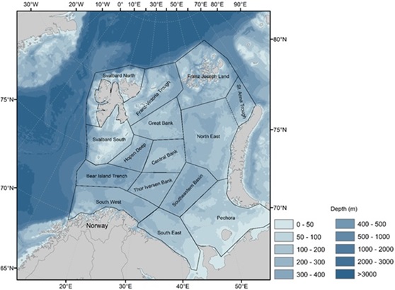
Målet med det felles norsk-russiske økosystemtoktet i Barentshavet og tilstøtende farvann, august-oktober (BESS) er å overvåke status og endringer i Barentshavets økosystem og skaffe data til bestandsrådgivning og forskning. Toktet har blitt gjennomført hvert år i samarbeid mellom Havforskningsinstituttet (HI) i Norge og VNIROs polaravdeling (PINRO) i Russland siden 2004. Den generelle toktplanen og undersøkelser ble avtalt på det årlige HI-PINRO-møtet i mars 2023. Båtruter og andre tekniske detaljer ble avtalt via korrespondanse mellom toktkoordinatorer. Toktet sikter på å dekke hele Barentshavet. Økosystemstasjonene er fordelt i et regelmessig rutenett (35×35 nautiske mil) og båtrutene følger dette designet med unntak av området rundt Svalbard med ekstra bunntråltrekk for et bedre estimat for bunnfisk og ekstra akustiske transekter for et beste estimat for loddebestandens størrelse.
Det 20. BESS-toktet ble gjennomført i perioden 10. august til 7. oktober av de norske forskningsfartøyene "Kronprins Haakon", "G.O. Sars" og "Johan Hjort", og det russiske fartøyet "Vilnyus". Som alltid vil vi takke mannskapet og det vitenskapelige personellet om bord på "Vilnyus", "G.O. Sars", "Kronprins Haakon" og "Johan Hjort" for deres innsats, samt til alle andre som har vært involvert i planleggingen og rapporteringen av BESS 2023.
Dette er første del av toktrapporten som oppsummerer observasjoner og statusvurderinger basert på toktdataene. Informasjonen fra BESS 2023 vil bli brukt videre til ulike internasjonale og nasjonale prosjekter, rapporter, vurdering av bestander av fisk og virvelløse dyr, miljøovervåking osv.
Del 1 dekker kapitlene 1 til 3, 5 til 7 og kap 9. Del 2 dekker de resterende kapitlene.
Summary
The aim of the joint Norwegian/Russian ecosystem survey in the Barents Sea and adjacent waters, August-October (BESS) is to monitor the status and changes in the Barents Sea ecosystem and provide data to support stock advice and research. The survey has since 2004 been conducted annually in the autumn, as a collaboration between the Institute of Marine Research (IMR) in Norway and the Polar branch of the VNIRO (PINRO) in Russia. The general survey plan and tasks were agreed upon at the annual IMR-PINRO Meeting in March 2023. Ship routes and other technical details are agreed on by correspondence between the survey coordinators. BESS aims at covering the entire Barents Sea. Ecosystem stations are distributed in a 35×35 nautical mile regular grid, and the ship tracks follow this design. Exceptions are the area around Svalbard/Spitsbergen, some additional bottom trawl hauls for demersal fish survey indices estimation, and additional acoustic transects for the capelin stock size estimation.
The 20-th BESS was carried out during the period from 10th August to 7th October by the Norwegian research vessels “Kronprins Haakon”, “G.O. Sars” and “Johan Hjort”, and the Russian vessels “Vilnyus”.
This is a first part of the survey report summarising the observations and status assessments based on the survey data. The information obtained in BESS 2023 will be further used for the implementation of various international and national projects, assessment of fish and invertebrate stocks, environmental monitoring, etc.
The aim of the joint Norwegian/Russian ecosystem survey in the Barents Sea and adjacent waters, August-October (BESS) is to monitor the status and changes of in the Barents Sea ecosystem. The survey has since 2004 been conducted annually in the autumn, as a collaboration between the IMR in Norway and the Polar Branch of VNIRO (PINRO) in Russia. The general survey plan, tasks, and sailings routes are usually agreed at the annual PINRO-IMR Meeting in March, but in 2023, due to external factors making physical meetings between Norwegian and Russian researchers difficult, they were agreed by correspondence. Survey coordinators in 2023 was Dmitry Prozorkevich (PINRO) and Geir Odd Johansen (IMR). No exchange of Russian and Norwegian experts between their respective ships in 2023. The 20-th BESS was carried out during the period from 10th August to 7th October by the Norwegian research vessels “Kronprins Haakon”, “G.O. Sars” and “Johan Hjort”, and the Russian vessels “Vilnyus”. The scientists and technicians taking part in the survey onboard the research vessels are listed in Table 1.
As always, we would like to express our sincere gratitude to all the crew and scientific personnel onboard RVs “Vilnyus”, “G.O. Sars”, “Kronprins Haakon” and “Johan Hjort” and for their dedicated work, as well as all the people involved in planning and reporting of BESS 2023.
This is a first part of the survey report summarising the observations and status assessments based on the survey data. The information obtained in BESS 2023 will be further used for the implementation of various international and national projects, assessment of fish and invertebrate stocks, environmental monitoring, etc.
Table 1.1 Vessels, participants and experts on each survey leg.
Research vessel
Participants
”Vilnyus” (10.08–28.09)
Pavel Krivosheya (Cruise leader, Pelagic fish), Alexey Amelkin (Demersal fish), Alexandr Pronuk (Pelagic fish), Alexey Rolsky (Demersal fish), Timofeu Mishin (Demersal fish), Denis Okatov (Instrumentation), Sergey Harlin (Instrumentation), Maksim Gubanishchev (Hydrologist), Alexey Kanischev (Hydrologist), Roman Klepikovsky (Sea birds and mammals), Marina Kalashnikova (Parasitologist), Kristina Hachaturova (Plankton, benthos), Alexandra Kudryashova (Plankton, Benthos).
“Kronprins Haakon” (15.09-6.10)
(15.09-06.10)
Elena Eriksen (Cruise leader), Heidi Gabrielsen (Benthos), Silje Seim (Demersal fish), Åse Husebø (Demersal fish), Susanne Tonheim (Pelagic fish), Erling Boge (Pelagic fish), Jan Henrik Simonsen (Plankton), Ragni Olssøn (Benthos), Elise Eidset (Demersal fish), Celina Eriksson Bjånes (Demersal fish), George McCallum (Marine mammals observer), Anna Tiu Kristina Simlia (Marine mammals observer), Asgeir Steinsland (Instrument chef ation), Hans Kristian Eide (Instrumentation), Monica Martinussen (Plankton), Berengere Husson (cruise leader under training), Arild Folkvord (Scientist guest, UiB), Jacob Max Christensen (Scientist guest, UiT), Joan Soto-Angel (Scientist guest, UiB), Jon Ford (Sea bird observer)
”G.O. Sars” (19.08–17.09)
Part 1 (19.08-01.09)
Edvin Fuglebakk (Cruise leader), Alexander Plotkin (Benthos), Else Holm (Demersal fish), Magne Olsen (Demersal fish), Adam Custer (Pelagic fish), Stine Karlson (Pelagic fish), Monica Martinussen (Plankton), Ida Vee (Benthos), Irene Huse (Demersal fish), Vidar Fauskanger (Demersal fish), Thomas André Sivertsen (Marine mammals observer), Lars Kleivane (Marine mammals observer), Sverre Waardal Heum (Instrumentation), Jan Frode Wilhelmsen (Instrumentation), Eli Gustad (Plankton), Gary Elton (sea bird observer)
Part 2 (01.09-17.9)
Rupert Wienerroither (Cruise leader), Mette Strand (Benthos), Anne Kari Sveistrup (Benthos), Sigmund Grønnevik (Demersal fish), Arne Storaker (Demersal fish), Thomas André Sivertsen (Marine mammal observer), Lars Kleivane (Marine mammal observer), Jan Frode Wilhelmsen (Instrument chef), Egil Frøyen (Instrumentation), Hilde Arnesen (Plankton), Irene Huse (Demersal fish), Else Holm (Demersal fish), Vilde Regine Bjørdal (Pelagic fish), Inger Henriksen (Pelagic fish), Hege Skaar (Plankton), Thomas André Sivertsen (Marine mammals observer), Lars Kleivane (Marine mammals observer), Gary Elton (sea bird observer).
Author(s):
Dmitry Prozorkevich (PINRO-VNIRO) and Elena Eriksen
(IMR)
Figures by: S. Karlson and E. Bagøien
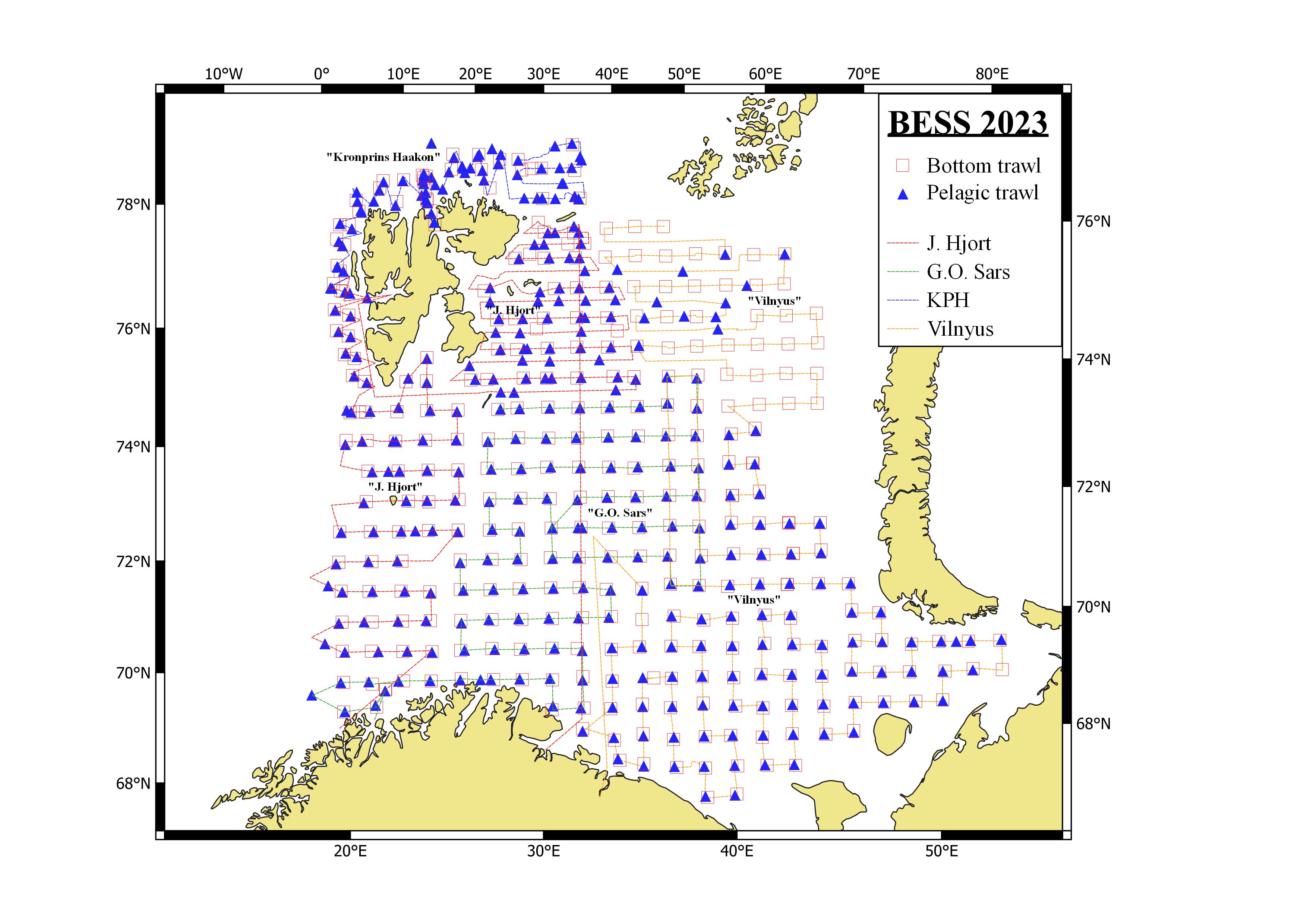
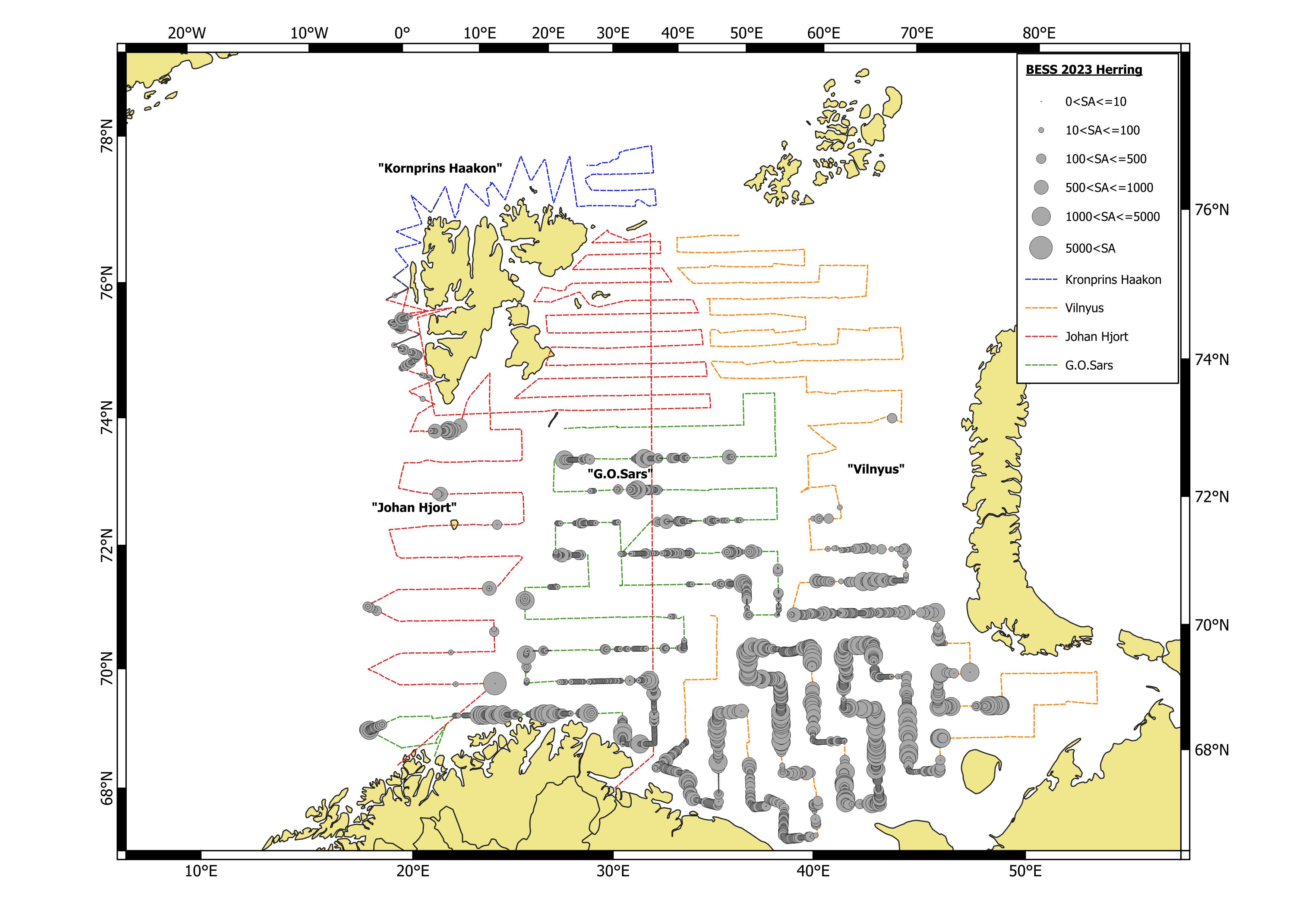
BESS aims to cover the entire ice-free area of the Barents Sea, from south to north. The ecosystem stations are distributed on a regular 35×35 nautical mile regular grid with the exception of the slope around Svalbard/Spitsbergen, with additional bottom trawl hauls for demersal fish indices estimation and additional acoustic transects east for Svalbard/Spitsbergen for the capelin stock size estimation. The planned vessel tracks for BESS 2023 are given in figure 2.1.
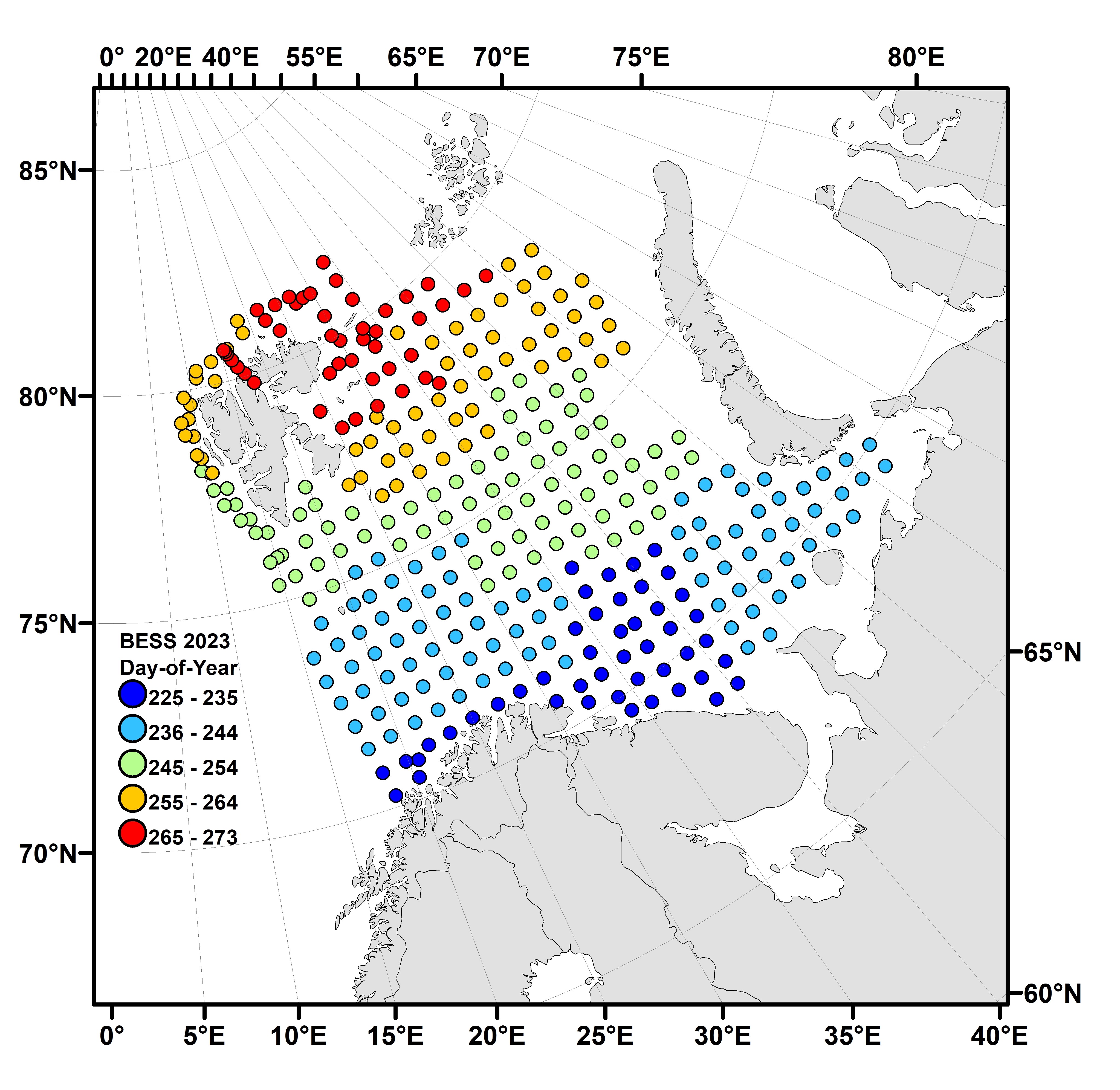
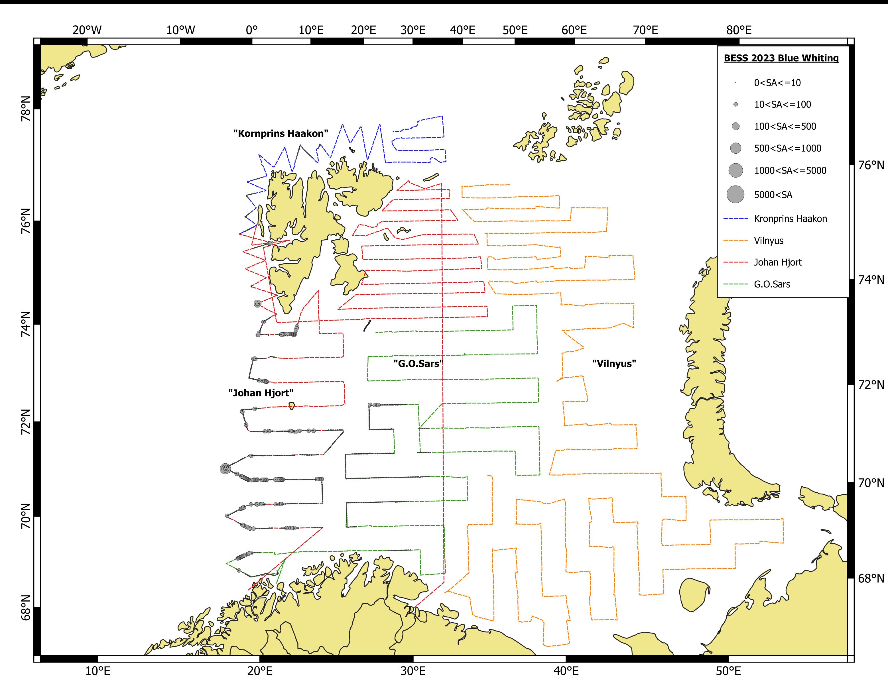
According to the plan, BESS 2023 was largely implemented. The realized tracks of the research vessel with the sampling taken are shown in Figures 2.2 and 2.3. The execution of BESS 2023 did not reveal any major changes or irregularities. The Russian vessel did not have enough allocated vessel-days to cover the region east of Franz Josef Land and in the north-eastern part of the survey area (Figures 2.2 and 2.3). A relatively large part of the Russian EEZ west of the Novaya Zemlya was closed for fishing at the request of the Russian Ministry of Defence, so survey area along the archipelago coast was not fully covered (Figure 2.2). For the same reason, some of the coverage of the Loophole has been moved from G.O. Sars part 1 to G.O. Sars part 2. A decrease in the number of standard pelagic trawls and reduced area coverage west of the Novaya Zemlya may lead to some underestimation of 0-group of cod, and significant underestimation of the polar cod stock size, including 0-group and juvenile Greenland halibut numbers. BESS 2023 was largely conducted according to the planned time schedule. In recent years, the number of ship days for a Russian vessel has been reduced with 10 %, while additional tasks (such as microplastic samples) have been added, leading to a reduction in survey area coverage. The planned schedule for BESS 2023 was 148 days (98 NOR+50 RUS), while the effective vessel days (time between first and last sample in the vessel logs) was 129 days (83 NOR+46 RUS). The difference between the two is as expected, as vessels need time for sailing to and from the harbor and preparation before sampling. The temporal and spatial progression during the survey was good (Figure 2.4). Weather conditions were very good for most of the period. Note that in reports from earlier years, only the planned schedule is reported.
The ecosystem survey in 2023 was similar to previous years, covering most ecosystem components. In addition to the standard coverage of most ecosystem components, the Norwegian vessels covered the oceanography sections “Vardø-Nord”, “Sørkapp-Vest”, and “Hinlopen” and the Russian vessel covered “Kola” section twice (Figure 2.3). During the BESS, a total of 362 pelagic hauls and 337 demersal were taken.
Figure 2.1. BESS 2023, planned survey map with ecosystem stations and vessel tracks.
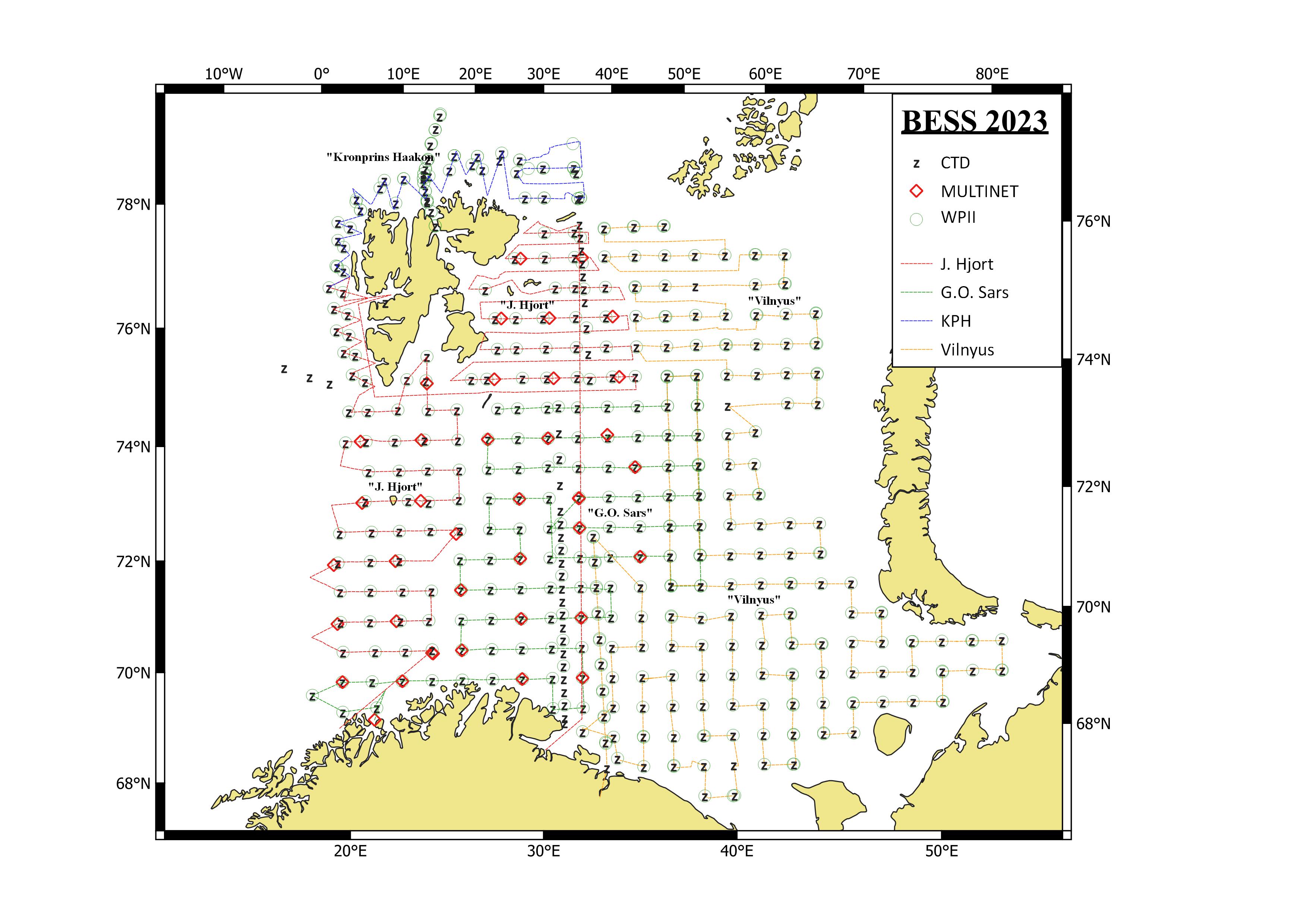
Figure 2.2. BESS 2023, realized vessel tracks with pelagic and bottom trawl sampling stations, note that some trawl stations are taken in addition to the regular ecosystem stations.Figure 2.3. BESS 2023, realized vessel tracks with hydrography and plankton samples at ecosystem stations.
Figure 2.4. Progression of BESS 2023 in space and time. Points represent samples taken at ecosystem stations during the survey. The point’s colour indicates the number of Julian days between the first and last day of the survey. The colours scale from blue (early in the survey) to red (late in the survey).
2.1 Sampling methods
In 2023, compared to 2022, there were no changes in sampling gear. Manta trawl was included as standard equipment for monitoring microplastics at BESS in 2022 and was also used in 2023. 47 samples were collected on Russian vessel and 25 on board Norwegian vessels. A new length stratified individual sampling of haddock, consisting of two fish taken for each 5 cm group, was started in 2022 and continued in 2023.
Plankton stations were carried out within the entire survey water area with sampling in the bottom-0 m layer. On the Kola hydrological section, plankton sampling collected separate for the layers: bottom-0 m, 100-0 m and 50-0 m.
The survey sampling manuals can be obtained by contacting the survey coordinators.
These manuals include methodological and technical descriptions of equipment, the trawling and capture procedures by the sampling tools, sampling and registration of the catch in the lab, and the methods that are used for calculating the abundance and biomass of the biota.
2.2 Special investigations
BESS is a useful platform for conducting additional studies in the Barents Sea. These studies can be testing of new methodology, sampling of data additional to the standard monitoring, or sampling of other types of data. It is imperative that the special investigations do not influence the standard monitoring activities at the survey. The special investigations vary from year to year, and below is a list of special investigation conducted on Russian and Norwegian vessels at BESS 2023, with contact persons. This chapter also briefly mentions some investigations that are typical during survey but not described in the main text of the BESS Report.
2.2.1 Annual monitoring of pollution levels
In 2023 PINRO continued the annual monitoring of pollution levels in the Barents Sea in accordance with a national program. Samples of seawater, sediments, fish and invertebrates was collected and analysed for persistent organic pollutants (POPs, e.g. PCBs, DDTs, HCHs, HCB) and heavy metals (e.g. lead, cadmium, mercury) and arsenic. The samples were collected at RV "Vilnyus" during BESS in the southern and eastern parts of the Barents Sea. The results from chemical analyses are available in the annual PINRO report “Status of biological resources…”.
2.2.2 Collection of samples for biochemical studies
Frozen samples of commercial and non-commercial fish and invertebrates were collected for biochemical studies (ratio of body parts, chemical composition of nutrients, molecular weight of muscle proteins, amino acids and lipid fractions composition) in accordance with a research program. Samples were frozen at a temperature -18°C immediately after catching before rigor mortis.
Contact: Kira Rysakova, PINRO-VNIRO (rysakova@pinro.vniro.ru)
2.2.3 Fish pathology research
PINRO undertakes yearly investigations of fish diseases in the Barents Sea (mainly in REEZ). 10 commercially important fish species (total 10 710 ind.) were studied. Red king crabs and snow crabs (total 387 ind.) were examined also for define “shell disease of crustaceans”. The main purpose of the pathology research is annual estimation of epizootic state of commercial fish and crabs species. The observations are entered into a database on pathology. This investigation was started by PINRO in 1999. Results are available in the annual PINRO report “Status of biological resources…”
In 2023, observations of the infestation of commercial fish species with helminths that are hazardous to human health continued on board the RV Vilnyus. Cod, haddock, polar cod, capelin, Atlantic herring place and LRD were examined in order to identify hazardous parasites. The results will be published later in PINRO annual report. Moreover, parasite larvae Pseudoterranova sp. from different areas of the Barents Sea were collected and fixed for further genetic studies.
2.2.5 Plankton and fish calorie content investigation
Plankton (copepods, hepreiids and euphausiids ) was also collected from a trawl net, which was attached to the upper frame of a mid-water trawl to assess the caloric content of prey items of commercial fish. Juvenile fish and macroplankton were also colled from pelagic trawl catches.
Contact: Anna Boyko, PINRO-VNIRO (syromolot@pinro.vniro.ru)
2.2.6 Hydrochemical observations
In August and September, hydrochemical observations were made onboard RV “Vilnyus” in the Kola section. Dissolved oxygen in the surface and bottom layers as well as biochemical oxygen demand during 5 days in the bottom layer were measured.
Contact: Alexander Trofimov, PINRO-VNIRO (trofimov@pinro.vniro.ru)
2.2.7 Fish diet study
Since 2004, investigations of diet of most abundant pelagic and demersal fish have been conducted annually during the BESS. In 2023 survey, onboard of Russian vessels stomachs of polar cod (374 stomachs), capelin (375 stomachs), cod (69 stomachs), haddock (203 stomachs), Greenland halibut (62 stomachs) and thorny skate (66 stomachs) were collected and frozen for detail analysis. In addition, express quantitative analysis of 3292 stomachs of 13 fish species (Atlantic herring, Kanin herring, capelin, polar cod, cod, haddock, long rough dab, Greenland halibut, plaice, deep-water redfish, golden redfish, thorny skate and spotted wolffish) was carried out. This analysis was done onboard RV “Vilnyus” during the cruise. Onboard of Norwegian vessels 706 stomachs of cod were collected and frozen for detailed analysis. In addition samples were collected and frozen for capelin, polar cod and Atlantic herring
Overview over special investigation taken on Norwegian vessels will be given in part 2 of the survey report.
3 - Data Management
Author(s):
Dmitry Prozorkevich (PINRO-VNIRO) and Elena Eriksen
(IMR)
3.1 Databases
A wide variety of data are collected during the ecosystem surveys. All data collected during the BESS are quality controlled and verified by experts Herdis Langøy Mørk and Elena Eriksen (IMR) and Tatyana Prokhorova (PINRO-VNIRO) during and after the survey. The data are stored in IMR and PINRO national databases, with different formats. However, the data are exchanged so that both sides have access to each other’s data and use equal joint data.
3.2 Data applications
The BESS aim to cover the whole Barents Sea ecosystem geographically and provide survey data for commercial fish and shellfish stock estimation. Stock estimation is particularly important for capelin, because capelin TAC is based on the survey result, and the Norwegian-Russian Fishery Commission determines TAC immediately after the survey. In addition, a broad spectrum of physical variables, ecosystem components and pollution are monitored and reported. The survey data will be used by each party for various purposes within the framework of national and international programs.
This survey report is based on joint data and contains the main results of the monitoring. The survey report will come in two parts and will be published in the IMR/PINRO Joint Report series.
All reports from BESS from 2004 until the latest are available at this web site: https://imr.brage.unit.no/imr-xmlui/handle/11250/2658167. This report is published in the IMR digital report series Joint IMR/PINRO Reports.
3.3 Time series of distribution maps
The redesigned IMR web site for the joint Norwegian/Russian Barents Sea Ecosystem Surveys is still not finished. The maps from this report series are to be made public in this map site when ready.
4 - Marine Environment
Ch. 4 Marine Environment is published in
Survey report (Part 2) from the joint Norwegian/Russian Ecosystem Survey in the Barents Sea and the adjacent waters August-October 2023
5 - Plankton Community
Author(s):
Sarah Joanne Lerch
, Elena Eriksen
, Berengere Husson
(IMR), Andrey Dolgov (VNIRO-PINRO), Dmitry Prozorkevich (VNIRO-PINRO) and Tatiana Prokhorova (VNIRO-PINRO)
5.1 Phytoplankton
Text by S.J. Lerch
Figures by S.J. Lerch
Samples used to characterize phytoplankton community composition and abundance were collected from a total of 108 stations over the course of four separate cruises. Samples were collected from Hinlopen and Vardø-Nord Utvidet during the ecosystem cruise (cruise numbers: 2023007016, 2023002011) between September and October, and Fugløya-Bjørnøya during transect cruises conducted in April (2023006008), May (2023002007), and August (2023002010). Microscopy was used to identify and quantify taxa in 39 preselected stations along the transects, covering multiple ICES sub-regions (Figure 5.1.1). Algae-net and metabarcoding samples were also collected which can be used to qualitatively assess community composition. In total, 28 Algae-net and 67 metabarcoding samples were collected.
Samples for algal cell counts (100 ml) were taken from 10 m CTD collected water and fixed in Neutral Lugol. Microscope counts were performed following the Utermöhl (1958) method on CTD samples to quantify abundance and community composition at the IMR Flødevigen Plankton Laboratory. Qualitative Algae-net samples were collected using a vertical net tow (10 μm mesh; 0.1 m2 opening; 30-0 m), fixed with 2 ml 20% formalin and stored for future use. Metabarcoding samples were collected by filtering approximately 2 L of seawater, pre-filtered with 180 µm mesh, on to 25 mm filters with a pore size of 5 µm. Samples were then stored at -80 °C for future DNA extraction and sequencing.
Microscopy algal counts include heterotrophic and autotrophic groups, these communities will therefore be referred to as microplankton in the summarized results below.
5.1.1 Results and discussion
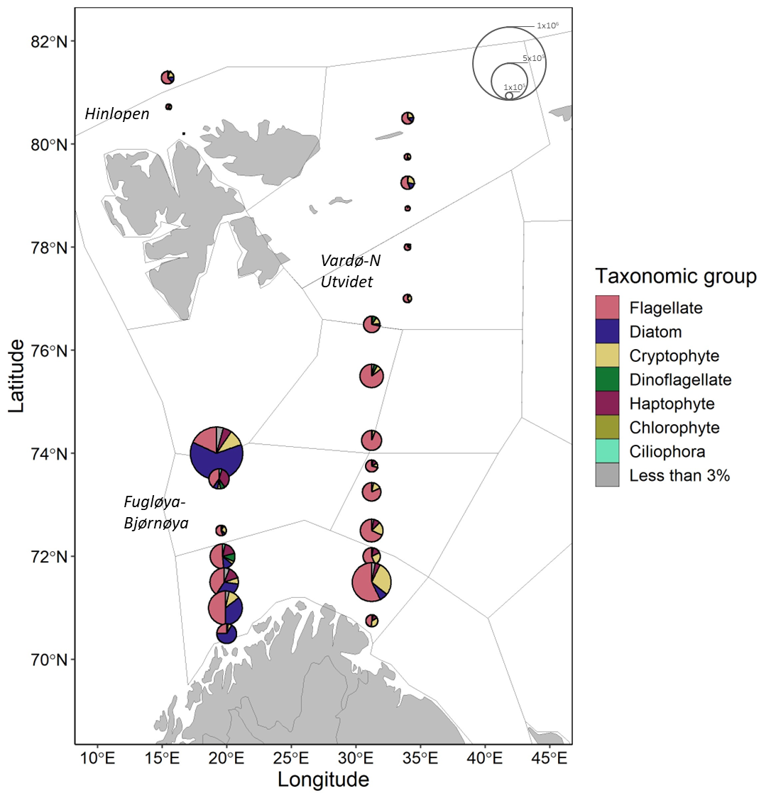
Based on microscopy counts, the average concentration of Barents Sea microplankton in the late summer/ early fall (August-October) was 3.41×10⁵ ± 2.25×10⁵ cells L-1. The average community was numerically dominated by flagellates (55%, 1.86×10⁵ ± 1.11×10⁵ cells L-1), diatoms (19%, 6.47×10⁴ ± 1.40×10⁵ cells L-1), and cryptophytes (15%, 5.10×10⁴ ± 4.24×10⁴ cells L-1).
Microplankton abundances and communities varied spatially across the Barents Sea in the late summer/ early fall (Figure 5.1.2). Cell concentrations varied by nearly two orders of magnitude between stations with a minimum concentration of 3.50×10⁴ cells L-1 and maximum of 1.01×10⁶ cells L-1. Higher concentration stations were generally found south of 74°N. The majority of Vardø-Nord and Hinlopen communities were flagellates and cryptophytes, while the Fugløya-Bjørnøya stations had large contributions from diatoms in addition to flagellates.
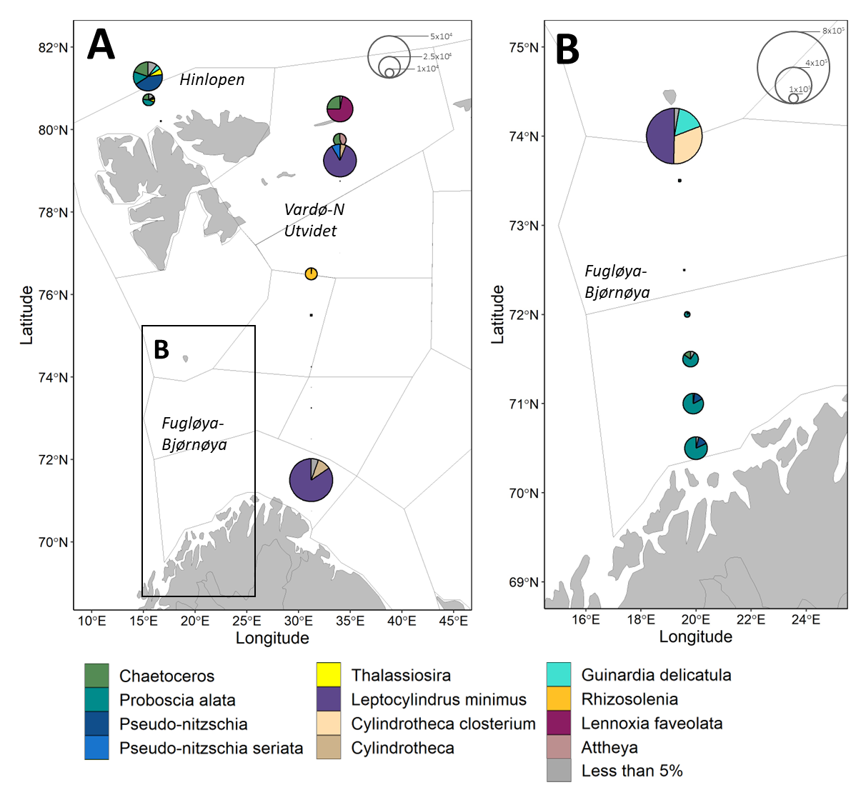
Within these data, diatoms are the only purely photosynthetic group described at a high taxonomic level. During the late summer/ early fall, diatom abundance was greatest near Bear Island and diatom community composition varied spatially (Figure 5.1.3). Leptocylindrus minimus comprised a large proportion of the community at multiple stations in Vardø-Nord and Fugløya-Bjørnøya. In addition, Probosica alata, Cylindrotheca Closterium and Pseudonitzschia are numerically important at some of the other stations with high diatom concentrations.
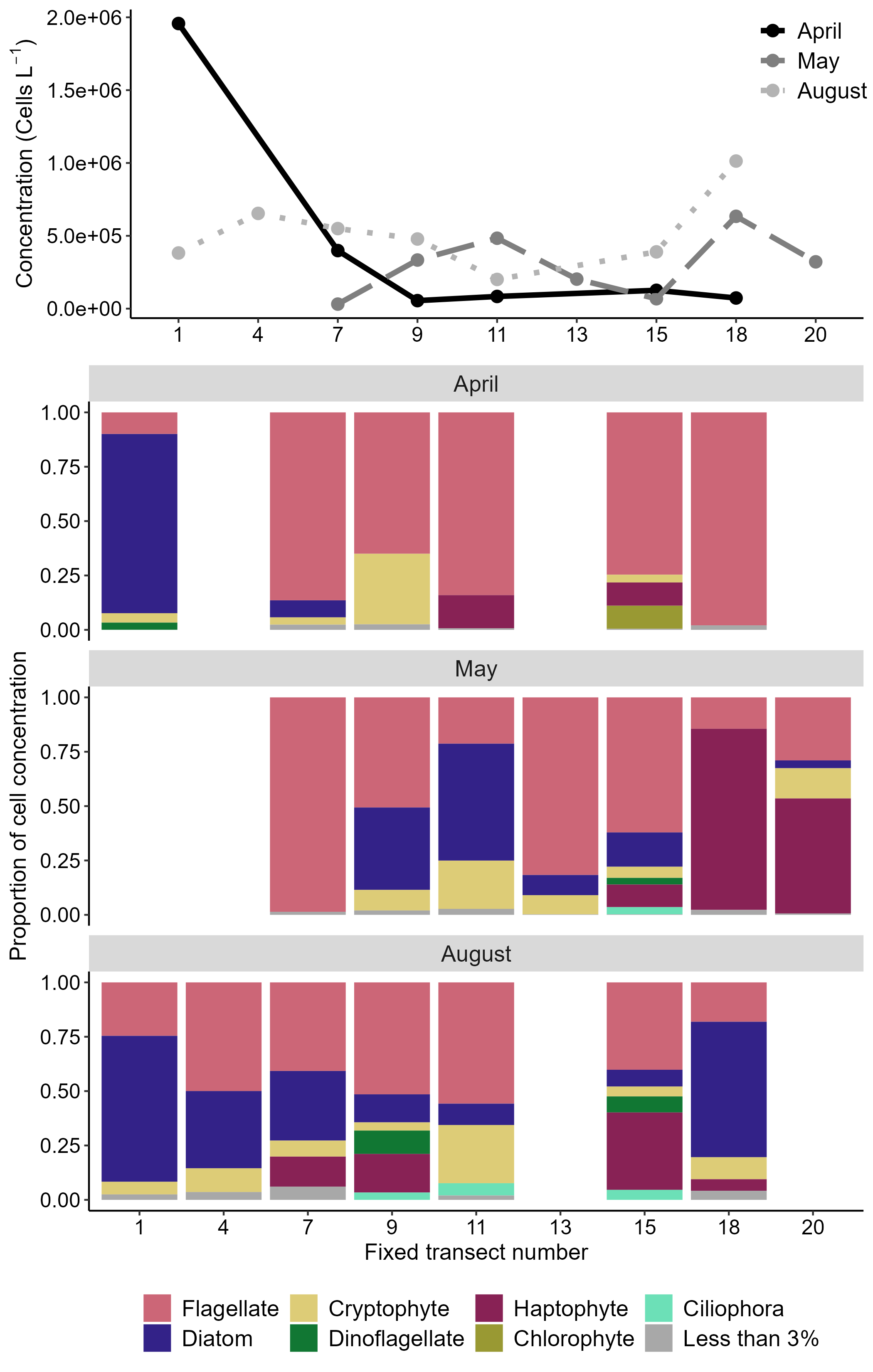
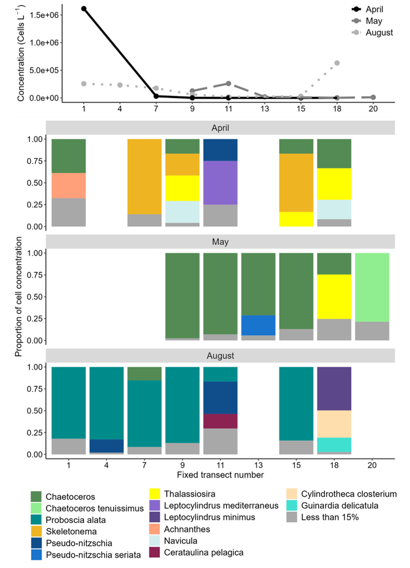
The combination of August and spring sampling along the Fugløya-Bjørnøya transect allows us to describe seasonal differences in microplankton cell concentrations and community composition. Average cell concentrations measured were the same order of magnitude in August (5.24×10⁵ ± 2.59×10⁵ cells L-1) and in the Spring (3.67×10⁵ ± 5.14×10⁵ cells L-1), although Spring samples were characterized by greater intra-station variability with particularly high cell concentrations at fixed station 1 in April (Figure 5.1.4). At the broad taxonomic group level, the Fugløya-Bjørnøya transect communities were variable with the only seasonal pattern being greater diversity and presence of diatoms across samples in August relative to the Spring (Figure 5.1.4). Diatom community composition shows clearer seasonal patterns (Figure 5.1.5). Chaetoceros and Thalassiosira were found almost exclusively in the spring and Skeletonema was found only in April. In contrast the August community was dominated by Proboscia alata and contained the only detection of Cerataulina pelagica, Cylindrotheca Closterium, and Guinardia delicatula.
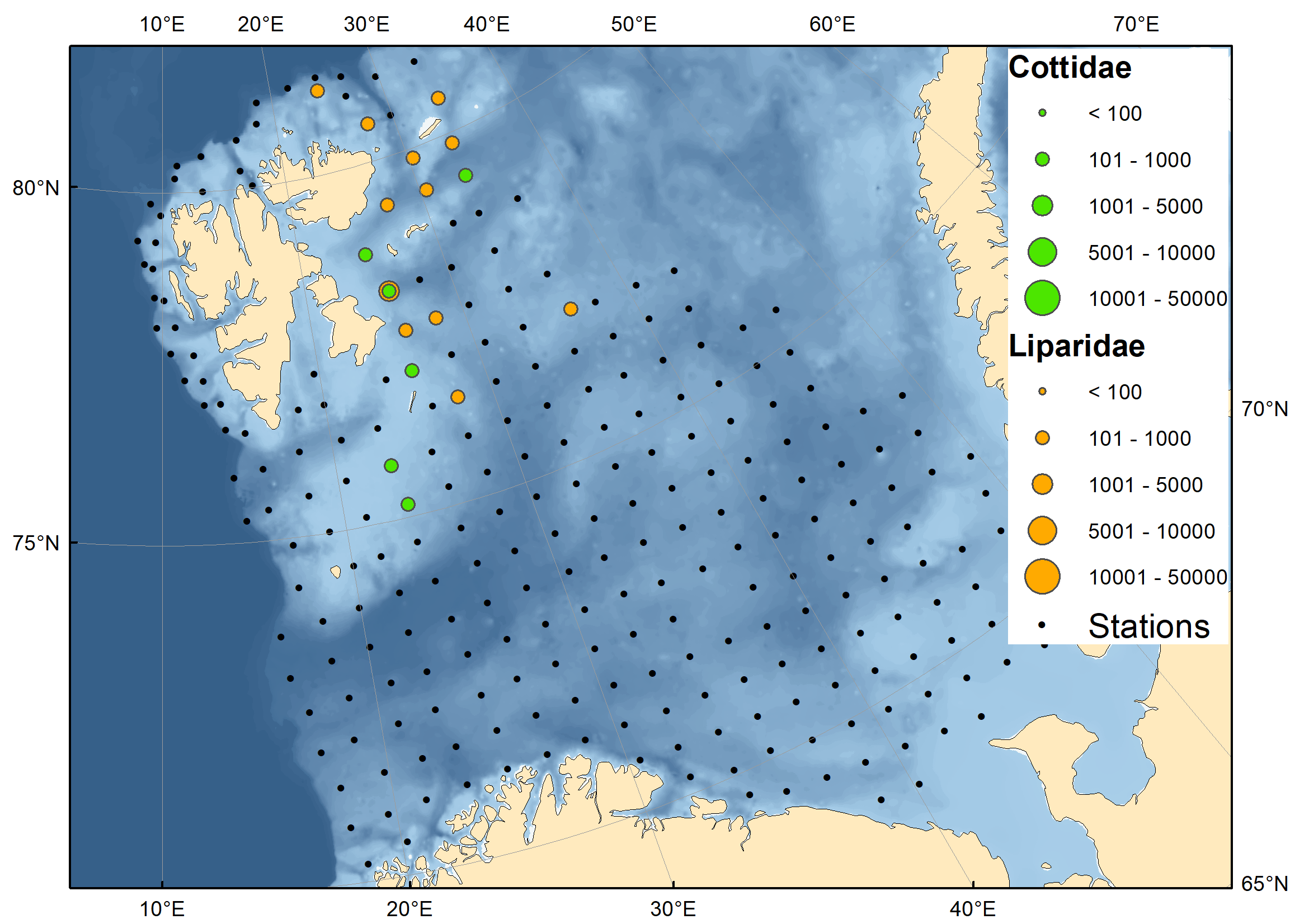
Figure 5.1.1. Map showing stations where phytoplankton samples were collected. Shapes indicate sampling activities at a given station: circle- metabarcoding sample collection, square- microscopy sample collection and analysis, star: algae-net sample collection. Color indicates the cruise when sampling occurred, blue: ecosystem, black: April transect cruise, dark gray: May transect cruise, and light gray: August transect cruise. Italicized labels indicate fixed transects. Outlined and labeled areas indicate ICES sub-regions. Sval-N: Svalbard North, Franz-Vic: Franz Victoria Trough, Sval-S: Svalbard South, HD: Hopen Deep, BI: Bear Island Trench, Th-Iv: Thor Iversen Bank, SW: South West. Station locations along Fugløya-Bjørnøya are shifted to reduce overlap of samples collected during separate cruises.Figure 5.1.2. Maps showing microplankton community composition and abundance for samples collected August-October 2023. Pie chart radii scale to cell concentrations in cells per liter based on key. Divisions within pie charts show the contributions from broad taxonomic groups. Italicized labels indicate fixed transects. All groups which comprised < 3% of the community are summed.
Figure 5.1.3. Maps showing diatom community composition and abundance for samples collected August-October 2023. A) Samples collected along Vardø-Nord and Hinlopen transects. B) Inset from A showing samples collected along Fugløya-Bjørnøya. Divisions within pie charts show taxonomic groups to the highest possible resolution. Pie chart radii scale to cell concentrations in cells per liter based on key. All groups which comprised < 3% of the community are summed.
Figure 5.1.4. Plots showing patterns in microplankton abundance (top) and community composition (bottom) along the Fugløya-Bjørnøya transect over three months in 2023. All groups which comprised < 3% of the community at a given station are summed for ease of visualization. Fixed station numbers increase as station locations move north.
Figure 5.1.5. Plots showing patterns in diatom abundance (top) and community composition (bottom) along the Fugløya-Bjørnøya transect over three months in 2023. Taxonomy is shown at the highest possible resolution. All groups which comprised < 15% of the community at a given station are summed for ease of visualization. Fixed station numbers increase as station locations move north.
5.2 Distribution and biomass indices of jellyfish
Text by E. Eriksen, D. Prozorkevich, T. Prokhorova and A. Dolgov
Figures by E. Eriksen
The biomass of gelatinous zooplankton was calculated using SAS (for the new 23 fisheries subareas, 1980-2017). The new 13 subareas, based on environmental status and bathymetry, were used from 2018 (Figure 6.2) to present spatial variation of jellyfish abundance and biomass. The R-script has been developed during the last three years, and during the last year some mistakes in the calculations were corrected. Thus, the biomass shown in previous reports may slightly differ from the latest one.
Here, we present the time series for biomass indices calculated by SAS (1980-2017) and by R (2018-2023). Spatial biomass indices calculated by R for 2004-2023.
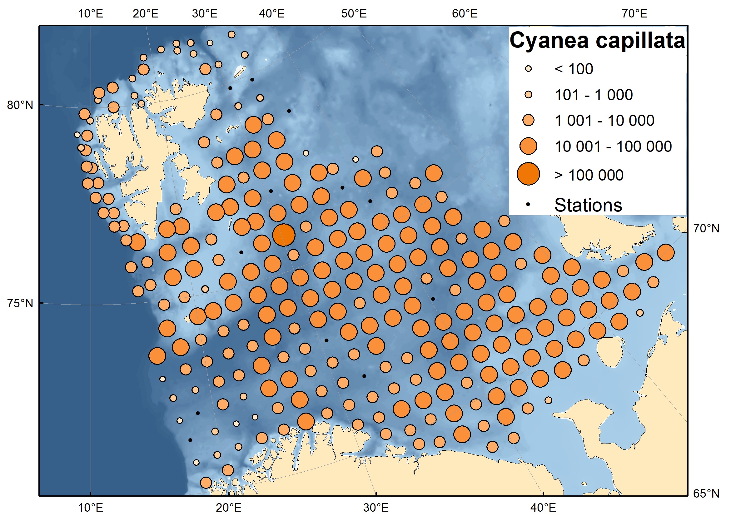
In August-October 2023, lion’s mane jellyfish (Cyanea capillata; Scyphozoa) was the most common jellyfish species, both with respect to weight (average density of 15.8 tonnes per nautical miles (nmi) and occurrence (found at 261 of 276 stations) (Figure 5.2.3.1). Higher densities (> 10 tonnes per sq nmi) were found widely in the Barents Sea (Figure 5.2.3.1).
Figure 5.2.3.1. Distribution of Cyanea capillata (wet weight; kg per nmi) in the Barents Sea, August-October 2023.
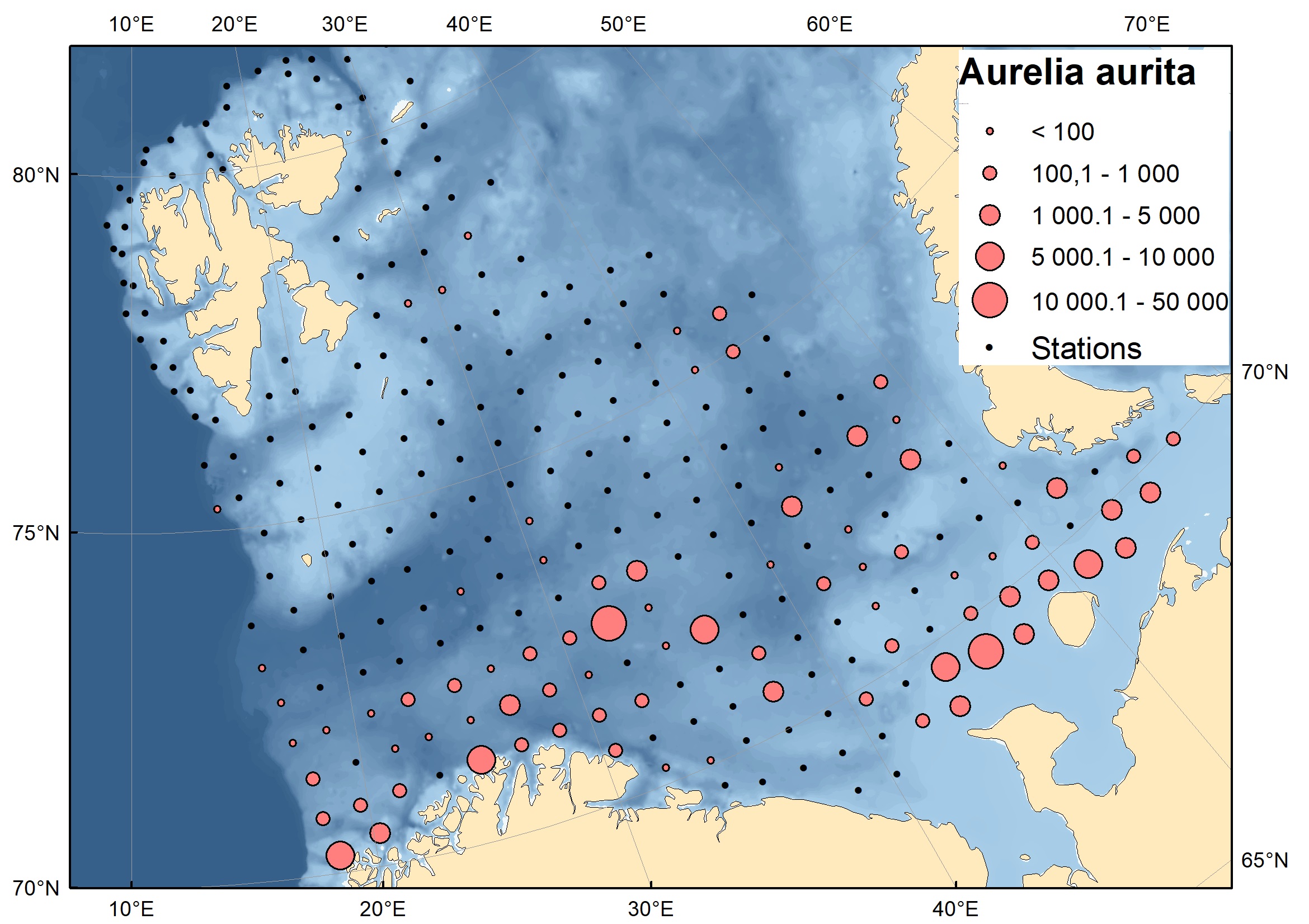
Moon jellyfish Aurelia aurita was found at 82 stations in the southern Barents Sea with an average biomass of 1 416 kg per nmi (Figure 5.2.3.2). Some few catches were also taken further north (3 stations), west (1 station) and east (4 stations).
Figure 5.2.3.2. Distribution of Aurelia aurita in the surveyed area in August-October 2023.
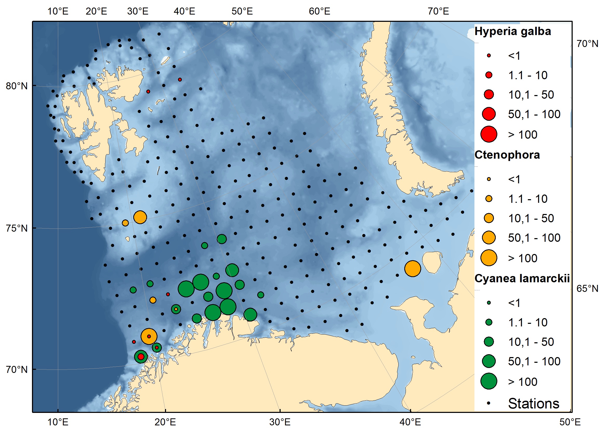
Blue stinging jellyfish, Cyanea lamarckii, was found at 19 stations in the western Barents Sea with average biomass 87.7 kg per nmi, which indicated an increase from earlier year (Figure 5.2.3.3). C. lamarckii has been observed regularly in the Barents Sea in recent years and the presence of this warm-temperate species may be linked to the inflow of Atlantic water masses.
Figure 5.2.3.3. Distribution of other jellyfish in the surveyed area in August-October 2023.
Ctenophores were found at 6 stations in the west and southeastern Barents Sea, with densities below 4 kg per sq nmi (3 stations) and above 80 kg (86, 157 and 233 kg per nmi), that was also unusual. Hyperiid amphipod Hyperia galba living into schiphoid jellyfish was found at 4 stations in southwest and two stations in the north with an average densities of 0.3 kg per nmi.
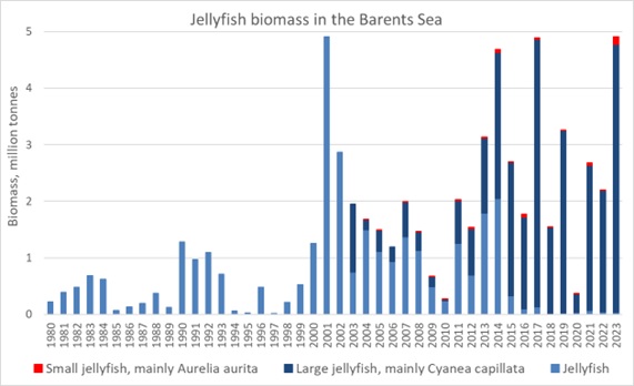
Biomass indices were calculated as total, for large jellyfish, dominating by C. capillata, small jellyfish dominating by A. aurita and undetermined jellyfish for the period 2004-2023. In 2023, total jellyfish biomass in the Barents Sea was similar to the record high in 2001 and was 4.905 million tonnes (Figure 5.3.3.3). Jellyfish biomasses dominated by biomasses of large jellyfish (4.743 million tonnes), although biomass of small jellyfish (dominated by A. aurita) was the highest recorded (130 thousand tonnes, Figure 5.2.3.4).
Figure 5.2.3.4. Total biomass of jellyfish in the Barents Sea in August-September 1980-2023. Large jellyfish were dominating by Cyana capillata, small jellyfish dominated by Aurelia aurita, and other jellyfish (found occasionally). Biomass estimates in 2018, 2020 and 2022 were underestimated due to lack of coverage.
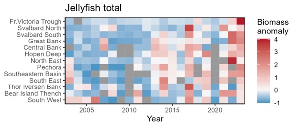
Geographical distribution of jellyfish, mainly C. capillata, showed an increase in central, southern, eastern, and northern areas since 2013 with the widest distribution in 2023, when biomasses reached almost 5 million tonnes (Figure 5.2.3.5).
Figure 5.2.3.5. Geographical distribution of jellyfish, mainly Cyana capillata in 13 polygons in August-September 2003-2023.
5.3 Distribution and biomasses of euphasiids and amphipods
5.3.1 Distribution and biomass of euphasiids
Text by E. Eriksen, B. Husson, A. Dolgov, D. Prozorkevich and T. Prokhorova
Figures by B. Husson and S. Karlson
Biomass estimates were calculated by different softwares during the last four decades: Excel (up to 2017) and R (since that). The new 15 subareas, based on similar environmental status, were used since 2018 (Figure 5.3.1.1). These areas were used to get more detailed information about the distribution of the krill within the survey area. The main differences between these two sets of estimates were that Excel used the average biomass of all stations to calculate the total biomass, while R used the average biomass for each of the 15 subareas and thus reducing the impact of single very high catches. In addition, sun elevation was calculated in R using getSunlightPosition script. The biomass estimates do not differ significantly due to the use of different software. The R-script for biomass estimation has been developed during the last three years, and last year some flaws were corrected. Thus the biomass values shown in previous reports may differ slightly from the previous ones.
Figure 5.3.1.1. Map showing subdivision of the Barents Sea into 15 subareas (polygons) used to estimate abundance of 0-group fish based on the BESS.
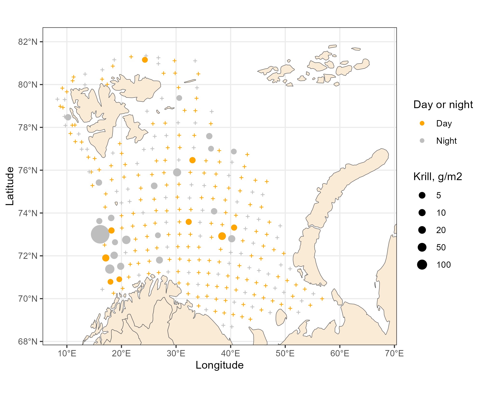
In 2023, euphausiids, also known as krill, were widely distributed in the western and central Barents Sea with higher abundance in the southwest (Figure 5.3.1.2). The biomass values in the upper 60 m are presented as grams (wet weight) per square meter (g/m2). In 2023, the night catches (mean 1.97 g/m2), were much lower than long term mean (7.3 g/m2).
Figure 5.3.1.2. Krill distribution, based on pelagic trawl stations covering the upper water layers (0-60 m), in the Barents Sea in August-October 2023.
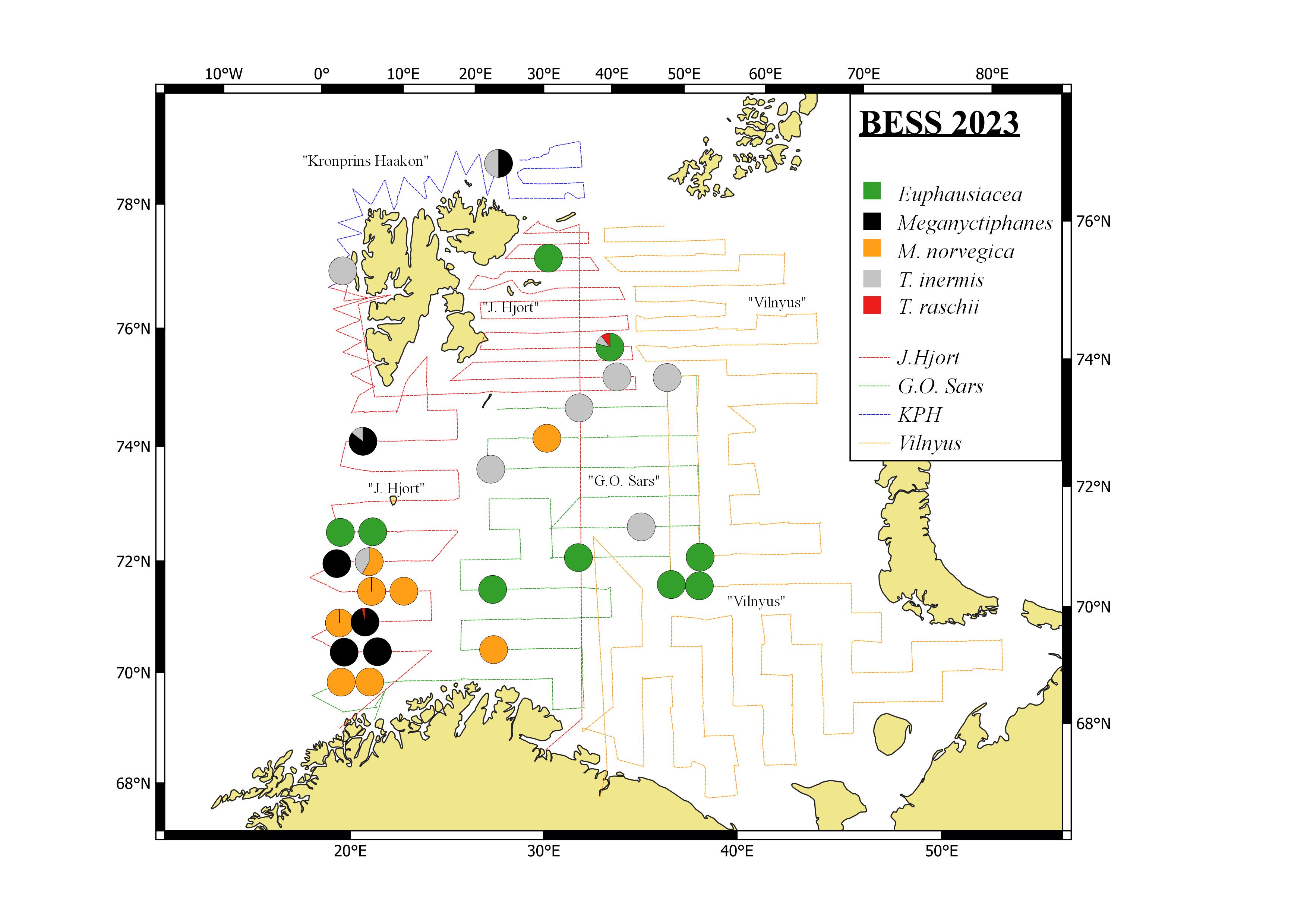
Based on the euphausiid species identification in 2023, Meganyctiphanes norvegica and were mostly restricted to the Atlantic waters in the southwest, while Thysanoessa inermis were mainly observed in the central and northern areas. Two catches of Thysanoessa raschii were taken in the southwest and one in the Great Bank (Figure 5.3.1.3). The smaller T. longicaudata were not found in 2023.
Figure 5.3.1.3. Krill species distribution, based on pelagic trawl catches covering 0-60 m, in the Barents Sea in August-October 2023.
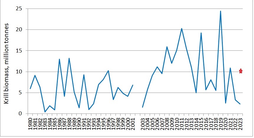
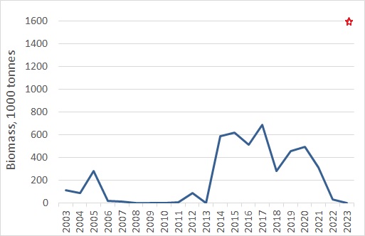
The number of night stations in 2023 was 108, while the day stations was 177. During the night, a majority of the krill populations migrate to the upper water layer for feeding and are therefore more available for the trawl. In the southwest one catch of 865.5 kg (corrected for trawl capture efficiency) was extremely high and thus influenced estimates of the total biomass of krill in the Barents Sea in 2023. The calculated total biomass of krill was 10.7 million tonnes with this catch (indicated with stars in Figure 5.3.1.4) and 2.3 million tonnes without this catch.
Krill were captured at fewer number of trawl stations than in previous years, and especially east of Svalbard/Spitsbergen and in the southern Barents Sea, indicating possible high predation pressure from capelin and young herring respectively.
Figure 5.3.1.4. Estimated total biomass of krill in the Barents Sea in August-October 1980-2023 based on pelagic night trawl catches covering the upper water layers (0-60 m). Estimates in 1980-2001 were calculated based on average night catches of all night stations and total surveyed area. Estimates in 2003-2022 were calculated based on an subarea average night catches and covered area within the subarea (Fig. 5.3.1.1). Estimates for 2002 are missing due to mistakes with the weight of krill. In 2023, one catch makes a big difference in estimates: total biomass with this catch (red star) and without blue line are shown.
5.3.2 Distribution and biomass indices of pelagic amphipods (mainly Hyeriids)
Text by E. Eriksen, B. Husson, A. Dolgov, D. Prozorkevich and T. Prokhorova
Figures by B. Husson and S. Karlson
Estimation of pelagic amphipods biomass for the Barents Sea was performed in R (see above) and presented here for the period 2003-2023.
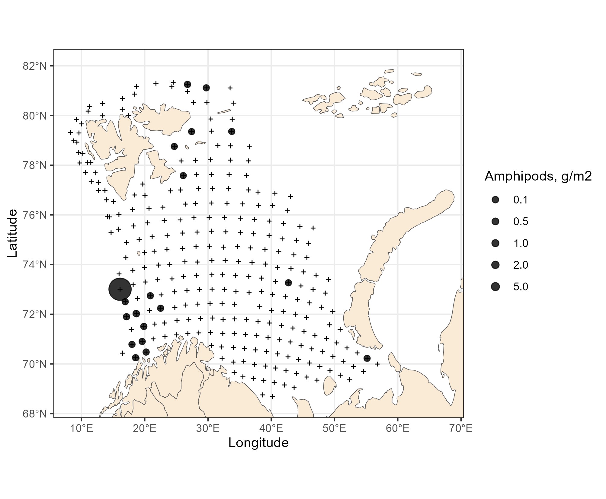
In 2023, amphipods generally occurred east off Svalbard/Spitsbergen and in the southwestern area (Figure 5.3.2.1).
Figure 5.3.2.1. Amphipods distribution, based on trawl stations covering the upper water layers (0-60 m), in the Barents Sea in August-October 2023.
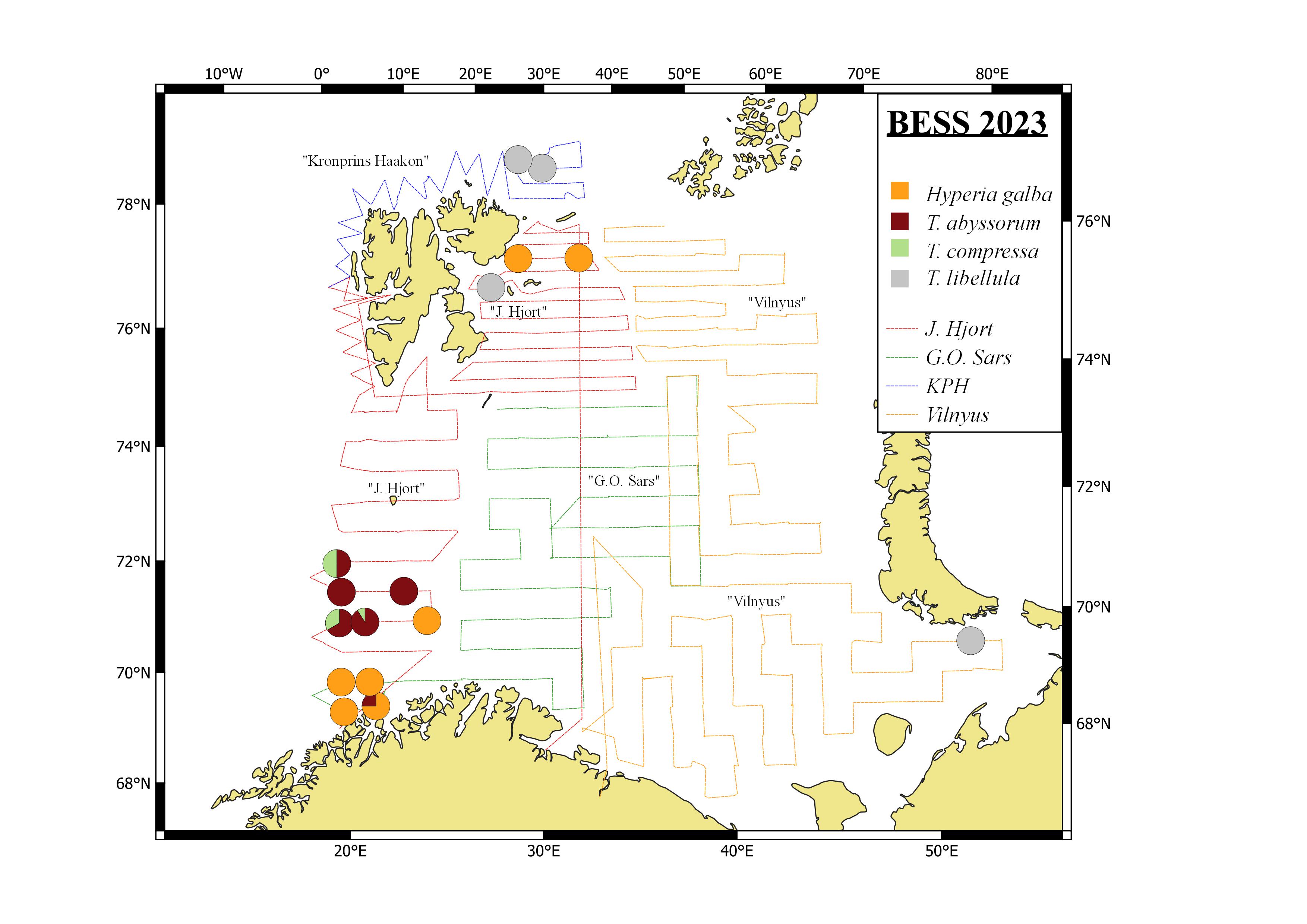
In 2023, amphipods taken east of Svalbard/Spitsbergen were mostly represented by the Arctic species Themisto libellula, while amphipods taken in southwest were mostly represented by subarctic Themisto compressa and Themisto abyssorum (Figure 5.3.2.2). The cosmopolitan species Hyperia galba were found in both areas. Smaller T. compressa (with max measured length of 13.0 mm) and T. abyssorum (with max measured length of 15.0 mm) are less captured by the trawl than larger T. libellula (with max measured length of 35.0 mm).
Figure 5.3.2.2. Distribution of pelagic amphipod species, based on pelagic trawl catches covering 0-60 m, in the Barents Sea in August-October 2023.
In the southwest, at one station, where the krill catch of 865.5 kg was taken, extremely high catch of amphipods of 389 kg (corrected for trawl capture efficiency) was also taken. This catch will have an impact on the total amphipod biomass in the Barents Sea in 2023, similar to the krill estimates. The calculated total biomass of amphipods in 2023 in the upper 60 m was 15.7 thousand tonnes with this catch and 1.08 thousand tonnes without this catch (Figure 5.3.2.3).
Figure 5.3.2.2. Estimated total biomass of pelagic amphipods in the Barents Sea in August-October 2023 based on pelagic trawl catches covering the upper water layers (0-60 m). Estimates in 2003-2022) were calculated based on a subarea’s average catches and covered area within the subareas (Figure 5.3.1.1). In 2023, one catch makes a big difference in estimates: total biomass with this catch (red star) and without (blue line) are shown.
6 - Fish Recruitment (young of the year)
Author(s):
Elena Eriksen
(IMR), Dmitry Prozorkevich (VNIRO-PINRO), Tatiana Prokhorova (VNIRO-PINRO) and Berengere Husson
(IMR)
Figures by: D. Prozorkevich
Area coverage and estimations
In 2023, the 0-group fish distribution was quite well covered by the survey (Figure 6.1).
Figure 6.1. Map showing spatial coverage of the 0-group fish in the Barents Sea in 2023. Dots indicate sampling stations colored according to research vessel, while grey lines denote the 15 subareas (polygons) used in the estimations.
Abundance and biomass estimates were calculated by different softwares during the last four decades: SAS (up to 2017), MatLab and R. The new 15 subareas, based on similar environmental status, was used from 2018 (Figure 6.2). They were included to get more detailed information about the distribution of the 0-group fish within the survey area. The abundance estimates do not differ significantly due to the use of different softwares. The R-script for abundance estimation has been developed during the last three years, and last year some mistakes in the calculations were corrected. Thus, the numbers and biomass shown in previous reports may slightly differ from the latest ones. Here, we present numbers of 0-group fish in million (106), billion (109) and trillion (1012).
Figure 6.2. Map showing subdivision of the Barents Sea into 15 subareas (polygons) used to estimate abundance of 0-group fish based on the BESS.
Total biomass
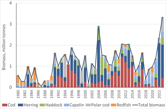
Zero-group fish are important consumers of plankton and are prey for predators (adult fish, sea birds and marine mammals) and, therefore, are important for the transfer of energy between trophic levels in the ecosystem. Estimated total biomass of 0-group fish species (cod, haddock, herring, capelin, polar cod, and redfish) varied from a low of 165 thousand tonnes in 2001 to a peak of 3.3 million tonnes in 2023, with a long-term average of 1.1 million tonnes for the period 1993-2023 (Figure 6.3). The estimated total biomass of 3.3 million tonnes in 2023 was record high. In 2023 like in 2004 and 2022, 0-group fish biomass was dominated by herring, and biomasses were higher than the long-term mean (period 1980-2023) for all species, except for redfish.
Figure 6.3. Biomass of 0-group fish species in the Barents Sea, August–October 1980–2023. The biomass of 0-group fish for the period 1980-1992 was estimated based on indices of total abundance and overall mean fish weight, and since then it has been estimated directly. Indices were calculated in SAS for the period 1980-2017 and in R since that. Biomass estimates for 2018, 2020 and 2022 were adjusted due to lack of survey coverage.
6.1 Capelin (Mallotus villosus)
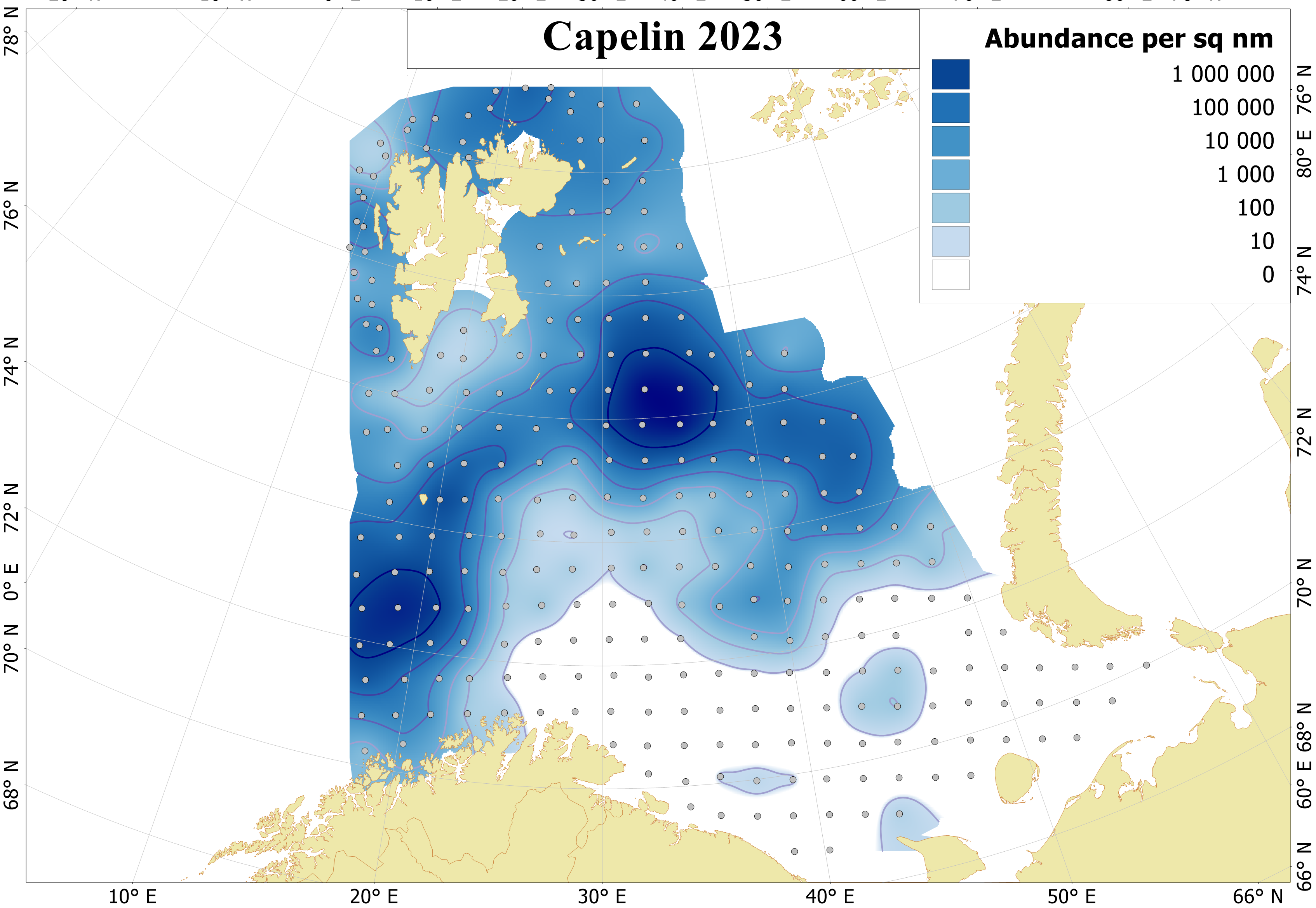
The highest average abundance was found in the Svalbard South (181 billion ind.), Great Bank (157 billion ind.), and Central Bank (139 billion ind.) polygons. The distribution of the 0-group capelin with little fish in the southeastern Barents Sea looks quite unusual compared to the long-term average (Figure 6.1.1). The lack of capelin in the southeast could be due to predation from the large number of juvenile herring in the area in 2023.
The 0-group capelin body length varied from 2.0 to 7.4 cm in 2023, while most of capelin (70%) were medium size with body length of 4.5-5.5 cm, which is similar to the length distribution in 2022. Larger individuals (with an average length above 5 cm) were found mainly in southeastern and northern areas, most likely indicating early spawning and drift to the rich feeding areas on the banks. The smallest capelin with average length close to 3 cm were found in the southwestern areas.
Figure 6.1.1. Distribution of 0-group capelin, August-September 2023. Abundance is corrected for capture efficiency (Keff). Dots indicate sampling locations.
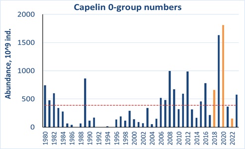
Two very strong year classes of capelin occurred in 2019 and 2020, followed by two below average year classes in 2021 and 2022, and now an above average year class in 2023. Estimated abundance of 0-group capelin has varied from 1 billion in 1993 to 1.8 trillion individuals in 2020 with a long-term average of 387 billion individuals for the 1980-2023 period (Figure 6.1.2). In 2023, the total 0-group capelin abundnace index (corrected for capture efficiency of the trawl) was 574 billion individuals which is above the long-term mean (Figure 6.1.2). The estimated biomass of 0-group capelin at 233 thousand tonnes was twice as high as the long-term mean. Therefore, the 2023 year-class of capelin seems to be middle-strong.
Figure 6.1.2. Estimated abundance of 0-group capelin corrected for capture efficiency (Keff) for the period 1980-2023. Red dotted line shows the long-term average. The abundance indices for 2018, 2020 and 2022 were adjusted due to lack of survey coverage and are shown in orange colour.
6.2 Cod (Gadus morhua)
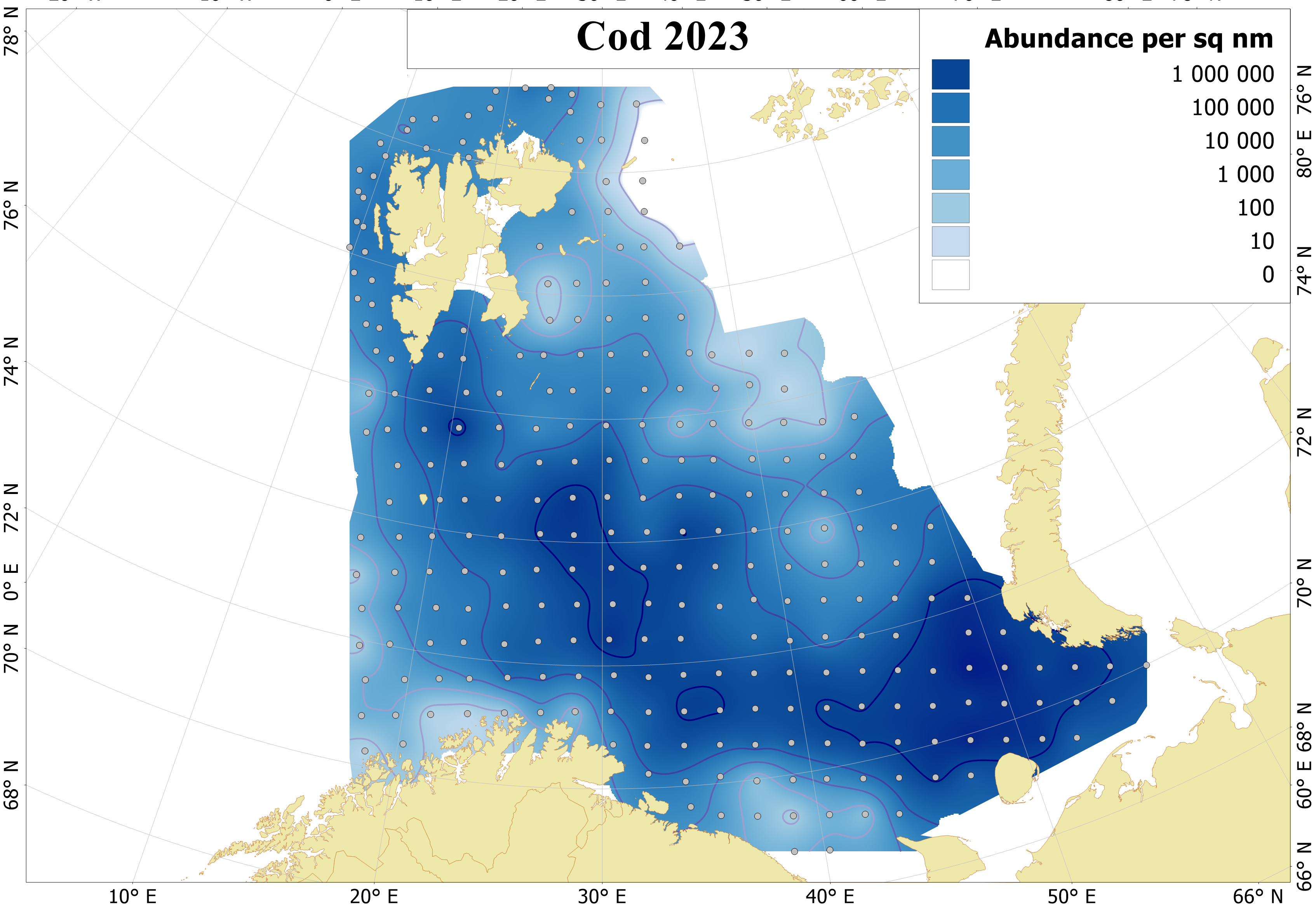
0-group cod were distributed widely in the BS, but the highest abundance was found in the southeastern (95 billion in Pechora) and north central (46 billion in Svalbard South) areas (Figure 6.2.1).
Figure 6.2.1. Distribution of 0-group cod, August-September 2023. Abundance is corrected for capture efficiency (Keff). Dots indicate sampling locations.
In 2023, 0-group cod were smaller than in 2022 and were dominated by fish of 5.0-7.4 cm length. The largest cod (with an average close to 8.0 cm) were observed in the northern polygons. Cod below 1.5 cm were found in the South West, Hopen Deep and Central Bank polygons.
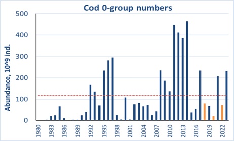
Estimated abundance of 0-group cod varied from 276 million in 1980 to 464 billion individuals in 2014 with a long-term average of 116 billion individuals for the 1980-2023 period (Figure 6.2.2). In 2023, the total 0-group cod abundance index (corrected for capture efficiency) was twice high as the long term mean and was 231 billion individuals. Cod estimated biomass in 2023 (440 thousand tonnes) was highest since 2017. Therefore, the 2023 year-class of cod could be characterized as strong.
Figure 6.2.2. 0-group cod abundance estimates corrected for capture efficiency (Keff) for the period 1980-2023. Red line shows the long-term average. Abundance indices for 2018, 2020 and 2022 were corrected for lack of coverage and shown by orange columns.
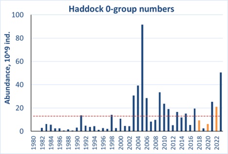
6.3 Haddock (Melanogrammus aeglefinus)
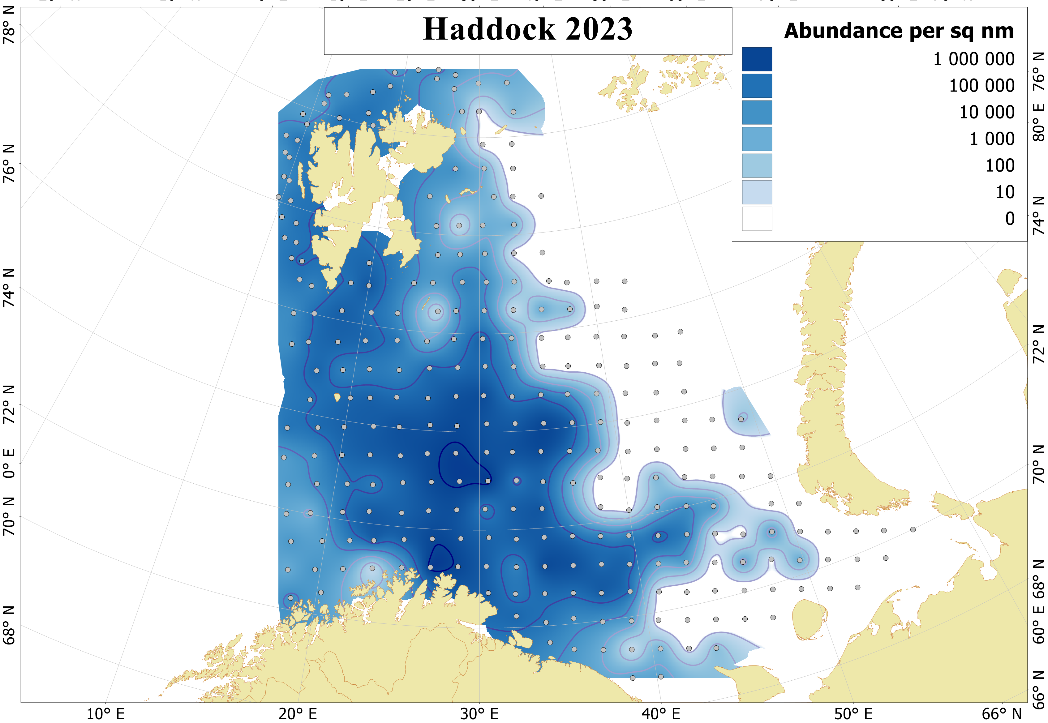
The 0-group haddock were found over a large area, with main abundance in the western areas – 15 billion in South West, and 10 billion in the Bear Island and in Thor Iversen Bank (Figure 6.3.1.).
Figure 6.3.1. Distribution of 0-group haddock, August-September 2023. Abundance are corrected for capture efficiency (Keff). Dots indicate sampling locations.
In 2023, 0-group haddock were dominated by fish from 7.0 to 9.4 cm. The largest haddock (with average length > 10 cm) were observed in the Central Bank and Svalbard North polygons, while smaller haddock were found in the Pechora and Franz Victoria Trough (with an average length < 8 cm). A very small 0-group haddock (below 2 cm) were found central areas, indicating later spawning.
Estimated abundance of 0-group haddock varied from 75 million in 1981 to 91.6 billion individuals in 2005 with a long-term average of 12.9 billion individuals for the 1980-2023 period (Figure 6.3.2).
Figure 6.3.2. 0-group haddock estimates corrected for capture efficiency (Keff) for the period 1980-2023. Red line shows the long-term average. Abundance indices for 2018, 2020 and 2022 were corrected for lack of coverage and shown by orange columns.
In 2023, the total 0-group haddock abundance estimates (corrected for capture efficiency of trawl) were higher than the long term mean and was 50 billion individuals. Haddock 0-group biomass in 2023 was estimated to 367 thousand tonnes and was the highest since 2009. Thus, the 2023-year class may be characterized as very strong.
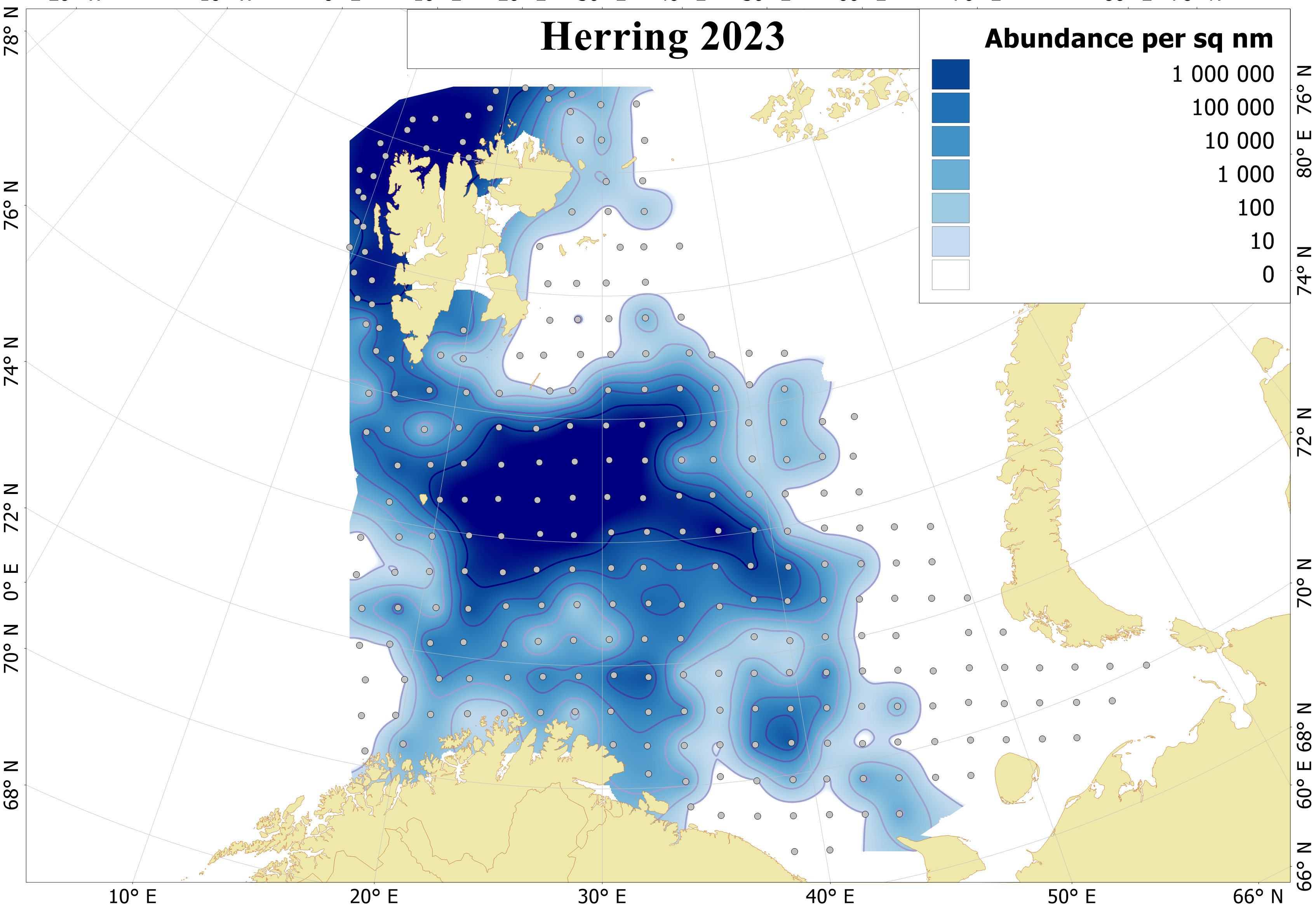
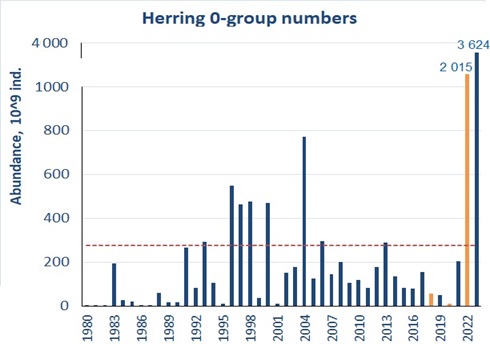
6.4 Herring (Clupea harengus)
0-group herring were widely distributed in the covered area, except in the eastern Barents Sea (Figure 6.4.1). The highest average abundance per station within a polygon was found in the Hopen Deep (2.3 trillion individuals). Relatively high abundance were also found in Svalbard South and Svalbard North and the Central Bank (with an average of 319-446 billion individuals).
Figure 6.4.1. Distribution of 0-group herring, August-September 2023. Abundance is corrected for capture efficiency (Keff). Dots indicate sampling locations.
The majority of 0-group herring (86%) had lengths in the range 4.5-6.5 cm, which is smaller than in 2022. Larger individuals were observed in Southeastern Basin with an average of 7.2 cm, while the smallest were found in the north central areas, where abundance was highest.
Figure 6.4.2. Estimated abundance of 0-group herring corrected for capture efficiency (Keff) for the period 1980-2023. Red dotted line shows the long-term average. Abundance indices for 2018, 2020 and 2022 were adjusted due to lack of survey coverage and are shown in orange colour.
Estimated abundance of 0-group herring varied from 37 billion in 1982 to a record high 3.6 trillion individuals in 2023 (Figure 6.4.2). Estimated biomass of 0-group herring at close to 1.7 million tonnes was lower than in 2022 and almost four times higher than the long-term mean (411 thousand tonnes). Therefore, the 2023-year class of herring may be characterized as record strong. Half of the 0-group herring abundance was distributed north of Svalbard/Spitsbergen and therefore their survival during the first winter is highly unknown.
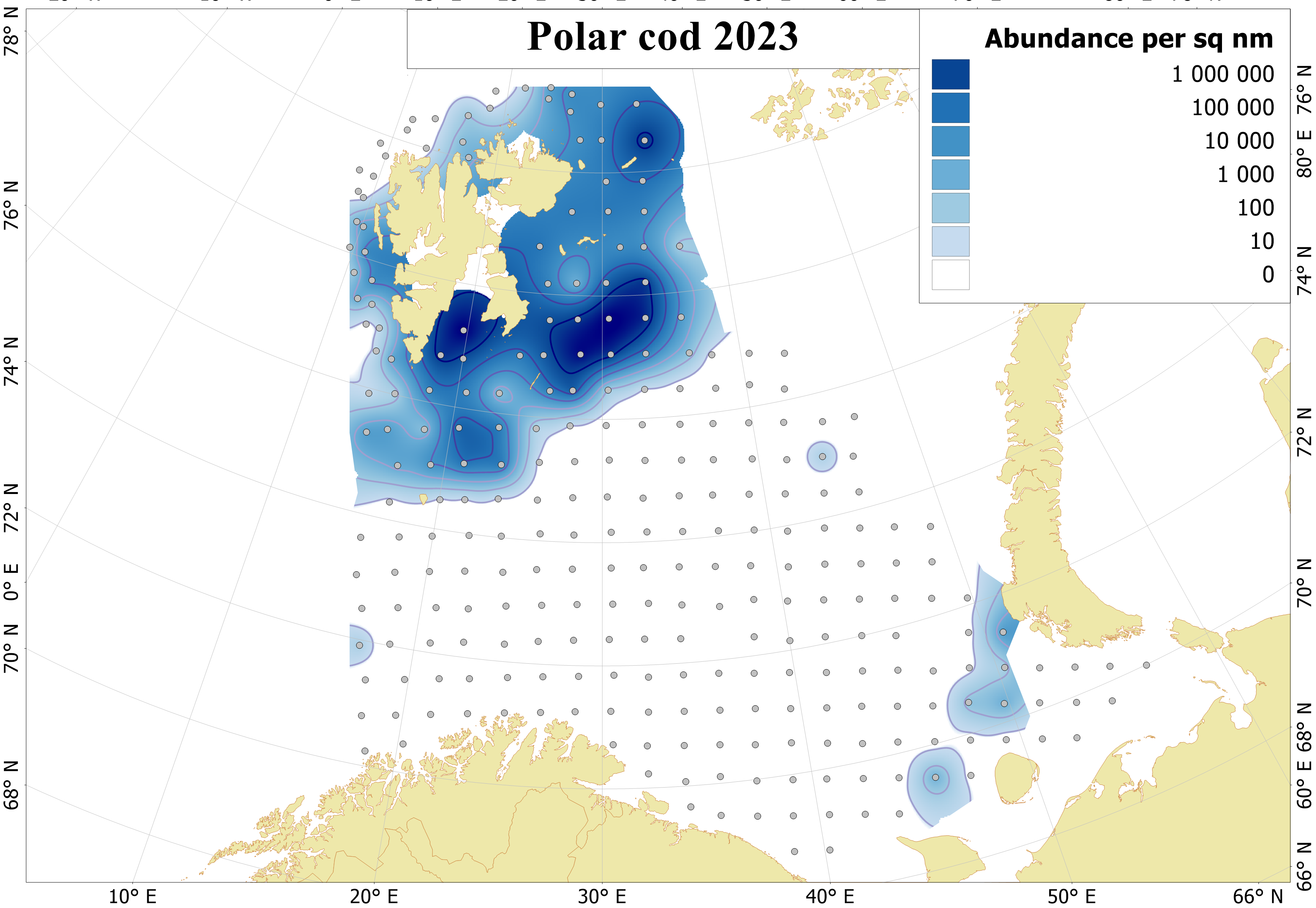
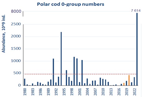
6.5 Polar cod (Boreogadus saida)
Polar cod 0-group were mainly found around Svalbard/Spitsbergen in 2023 which indicates that most of the spawning took place near this archipelago (Figure 6.5.1). The highest abundance was found in the Svalbard South polygon (with an average per station within the polygon of 2.4 billion individuals) and Great Bank polygon (with an average per station within the polygon of 3.6 billion individuals). A few polar cod were sampled in the southeastern Barents Sea, which indicated some spawning also there. For many years there was little or no spawning of polar cod in the Pechora area.
Figure 6.5.1. Distribution of 0-group polar cod, August-September 2023. Abundance is corrected for capture efficiency (Keff). Dots indicate sampling locations.
The length of 0-group polar cod varied between 0.5 and 8.0 cm, with fish in the length range 3.5-5.9 cm dominating. Average length was 5.1 cm. Average length varied between polygons and larger fish were found in the North East polygon (average of 6.5 cm), and smaller fish in the Pechora polygon (average of 3.6 cm).
Estimated abundance of 0-group polar cod varied from 201 million in 1995 to a record high 7.6 trillion in 2023 with a long-term average of 470 billion individuals for the 1980-2023 period. In 2023, the total abundance index for 0-group polar cod was the highest observed (Figure 6.5.2).
Figure 6.5.2. Estimated abundance of 0-group polar cod corrected for capture efficiency (Keff) for the period 1980-2022. Red dotted line shows the long-term average. Abundance indices for 2018, 2020 and 2022 were adjusted due to lack of survey coverage and are shown in orange colour.
In 2023, the estimated biomass of 0-group polar cod at 681 thousand tonnes was the second highest after 1994 and was more than four times higher than the long term mean of 147 thousand tonnes (1980-2023). For the first time since the observations started in 1980, the record strong year class originated mainly from the Svalbard/Spitsbegen sub-component.
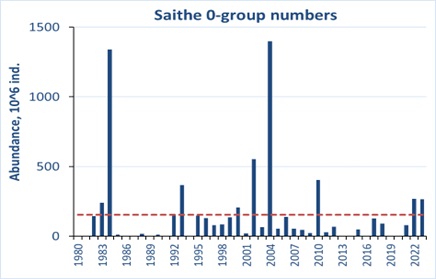
6.6 Saithe (Pollachius virens)
Saithe distribution and abundance varied a lot between years. In 2023, saithe were widely distributed, which is seldom observed (Figure 6.6.1).
Figure 6.6.1. Distribution of 0-group saithe in August-September 2023. Abundance is corrected for capture efficiency. Dots indicate sampling locations.
The largest saithe with an average of 11-12 cm were observed further north, while smaller fish (with an average of 8.6 cm) fish were found in the North East polygon.
Saithe abundance indices varied from some few hundred (1980 and 2020) up to 1 million individuals in 2004. During the last two years abundance of saithe were high and were 672 million (2022) and 342 million (2023), which are higher than in long term mean of 445 million individuals (Figure 6.6.1).
Figure 6.6.2. 0-group saithe abundance estimates corrected for capture efficiency for the period 1980-2023. Red line shows the long-term average.
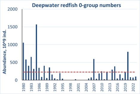
6.7 Redfish (mostly Sebastes mentella)
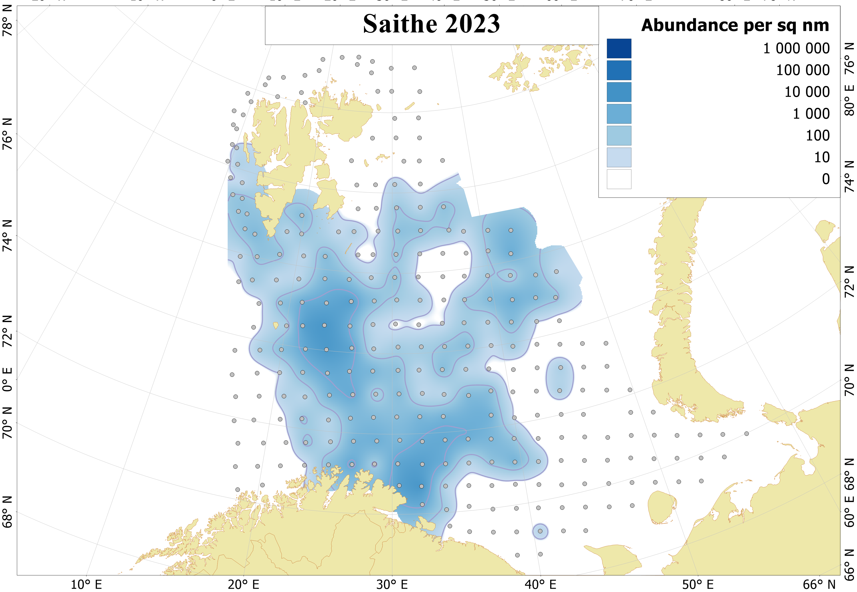
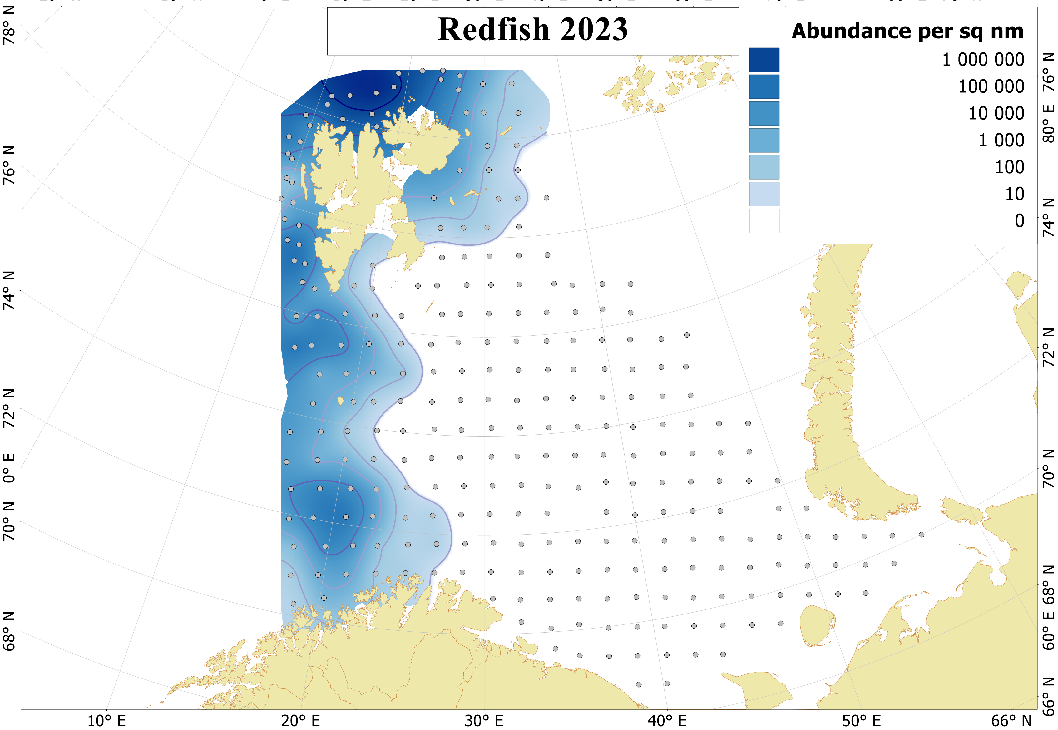
In 2023, 0-group redfish was distributed from north of Norwegian coast to Svalbard/Spitsbergen and around the archipelago, which is similar to the 2022 distribution (Figure 6.7.1). The highest abundance was found in Svalbard North (67 billion ind.) and Svalbard South (26 billion ind.) polygons. The largest fish with an average of 4.5 cm were found in the north, while smallest with an average of 2-3 cm were found in the south.
Figure 6.7.1. Distribution of 0-group redfishes (mostly Sebastes mentella) in August-September 2023. Abundance corrected for capture efficiency. Dots indicate sampling locations.
Estimated abundance of 0-group deepwater redfish varied from 23 billion individuals in 2001 to 1.6 trillion ind. in 1985, and long-term abundance was 229 billion individuals for the 1980-2023 period (Figure 6.7.2). In 2023, the total abundance index for 0-group deepwater redfish was half of the long term mean and was 102 billion individuals. The total biomass was close to 31 thousand tonnes. Thus the 2022-year class may be characterized as weak.
Figure 6.7.2. 0-group deepwater redfish abundance (corrected for trawl efficiency) in the Barents Sea during 1980-2023. Red line shows the long-term average.
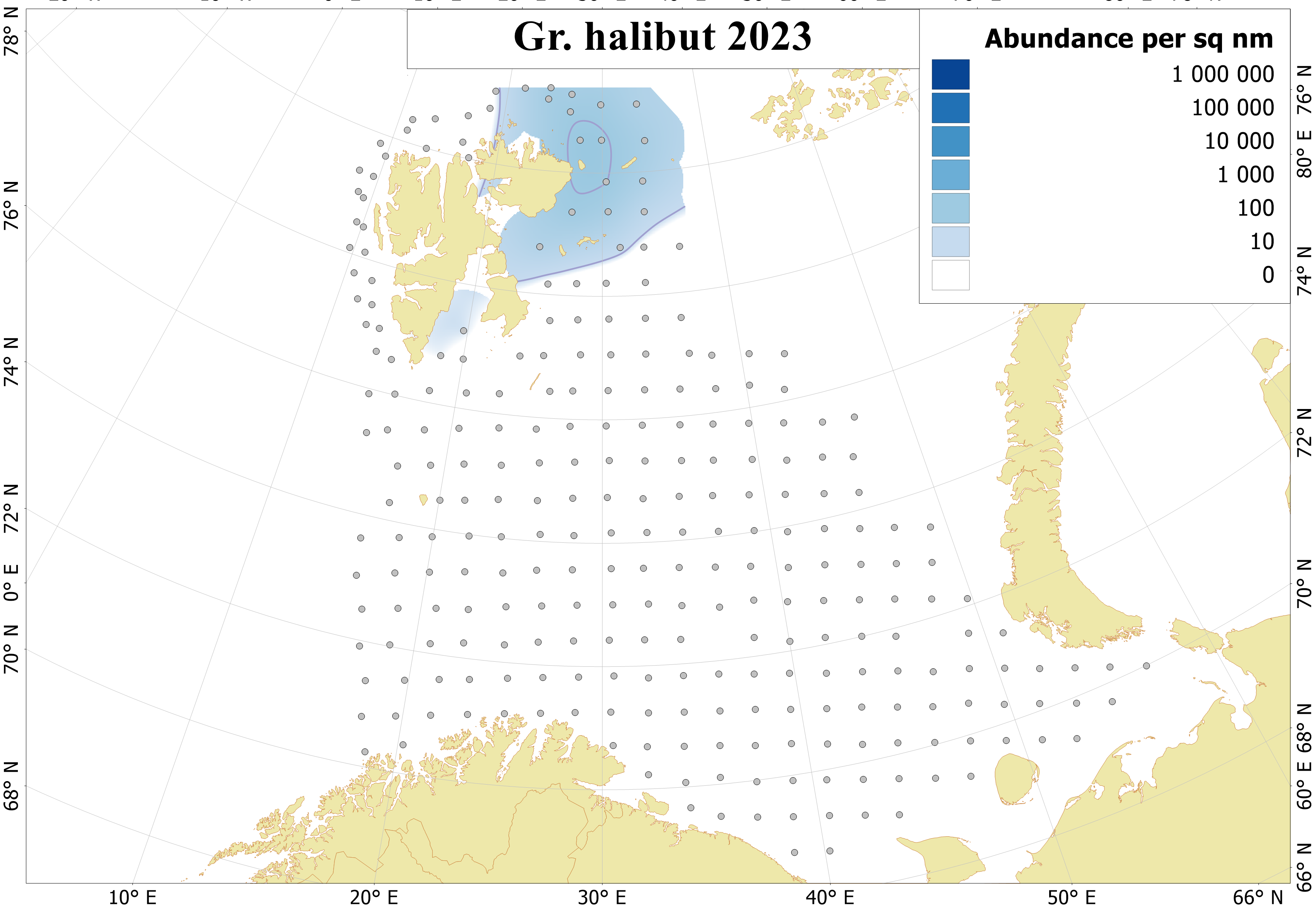
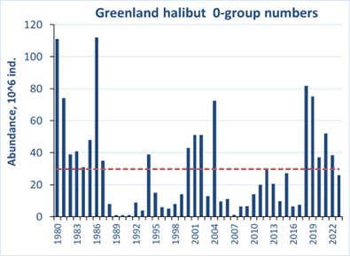
0-group Greenland halibut were found distributed around Svalbard/Spitsbergen in 2023, similar to the distribution in 2018-2022 (Figure 6.8.1). Highest abundance was found further north in Franz Victoria Trough polygon per square nautical miles.
An annual average length of 0-group Greenland halibut length was 6 cm than lower it in 2022 (7 cm). Fish length varied from 2.0 to 10 cm. The larger fish were found in Svalbard South with an average of 8 cm and smaller fish were found in the Franz Victoria Trough with an average of 5 cm.
Figure 6.8.1. Distribution of 0-group Greenland halibut, August-September 2023. Dots indicate sampling locations. Abundance not corrected for capture efficiency.
In 2023, the total abundance index for 0-group fish was 26 million individuals, that was lower than the last five years, and the long term mean of 30 million individuals. Estimated biomass was also lower than long term mean (of 80 tonnes) and was 35 tonnes.
Figure 6.8.2. 0-group Greenland halibut abundance estimates were not corrected for capture efficiency for the period 1980-2023. Red line shows the long-term average.
0-group Greenland halibut distributes widely in the North Atlantic and Svalbard/Spitsbergen fjords, therefore, abundance indices may not represent year classes strength, but give an indication of abundance in the Barents Sea. The 2022-year class may be characterized as weak but this is connected to high uncertainty due to the distribution pattern.
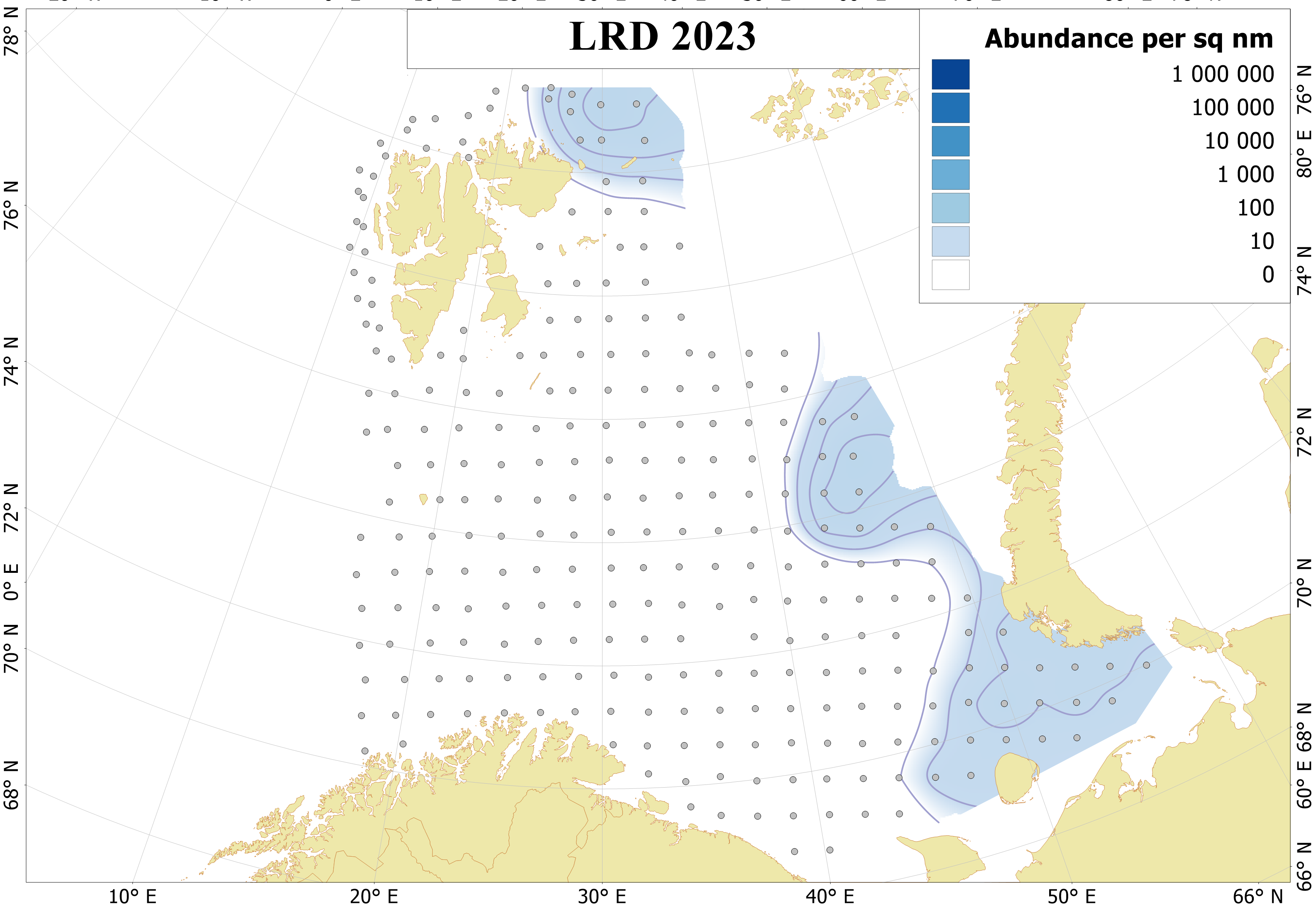
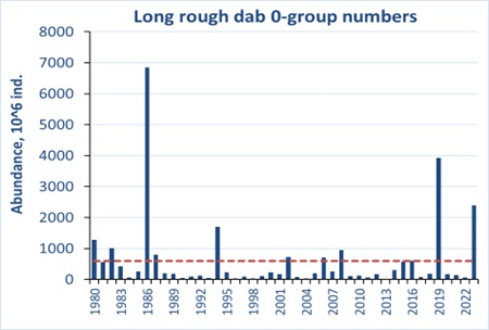
6.9 Long rough dab (Hippoglossoides platessoides)
In 2023, 0-group long rough dab were widely distributed in the Barents Sea (Figure 6.9.1). The highest densities were found in North East (an average of 51 thousand per square nautical miles) and the Southeastern Basin (an average of 46 thousand individuals per square nautical miles).
Figure 6.9.1. Distribution of 0-group long rough dab, August-September 2023. Dots indicate sampling locations. Abundance not corrected for capture efficiency.
The annual average length for 0-group long rough dab was 3.5 cm and was larger than the previous seven years. Fish length varied from 1 cm to 5.0 cm and larger fish (> 4 cm) were found in Great Bank and Franz Victoria Trough, while smaller fish (2.0 cm) in Pechora and North East.
In 2023, the total abundance index for 0-group fish was 2.4 billion individuals that was the largest since 2019 (Figure 6.9.2). Estimated biomass was higher than long term mean (of 297 tonnes) and was 720 tonnes.
Figure 6.9.2. 0-group long rough dab abundance estimates were not corrected for capture efficiency for the period 1980-2023. Red line shows the long-term average.
Thus the 2023-year class of long rough dab could be characterized as strong.
7 - Commercial Pelagic Fish
Author(s):
Georg Skaret
(IMR) and Dmitry Prozorkevich (PINRO-VNIRO)
The geographical distribution of capelin recorded acoustically is shown in Figure 7.1.1.1. Similar to last year, the capelin was distributed far north. The main distribution area was the Great Bank, which is typical late in the feeding season. Significant recordings were also made north and west of Svalbard/Spitsbergen, which is very unusual. The capelin recordings stretched towards east and north-east, and the recordings suggested that the distribution stretched even further north on the eastern side. Some capelin were recorded in the south-east, but apart from that, very little capelin were recorded south of 73°N.
Figure. 7.1.1.1 Geographical distribution of capelin in autumn 2023 based on acoustic recordings. Circle sizes correspond to NASC values (m2/nmi2) per nautical mile.
7.1.2 Abundance by size and age
A detailed summary of the acoustic stock estimate is given in Table 7.1.2.1, and the time series of abundance estimates is summarized in Table 7.1.2.2. A comparison between the estimates in 2023 and 2022 is given in Table 7.1.2.3 with the 2022 estimate shown on a shaded background.
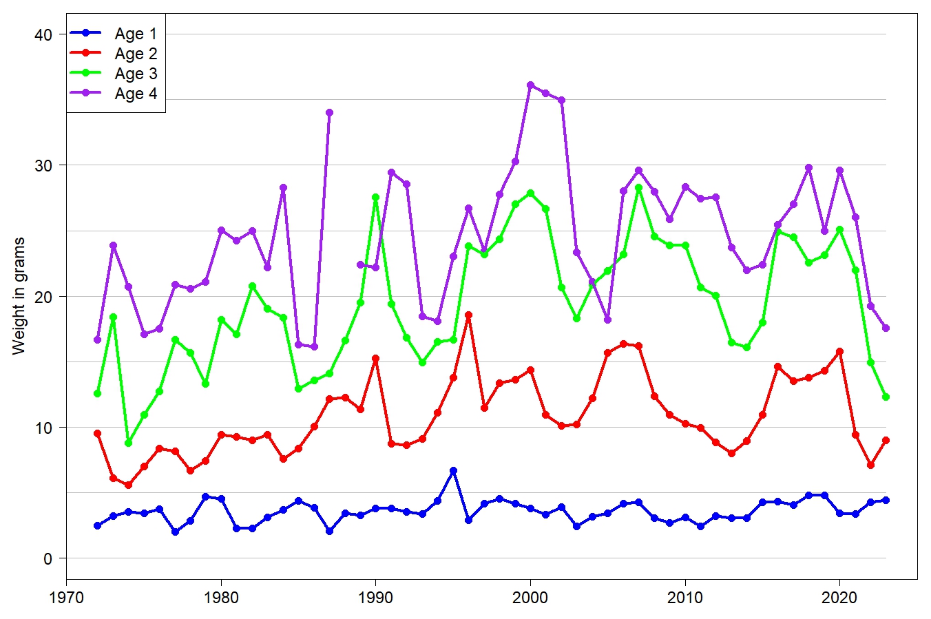
The total stock in the covered area was estimated to about 2.95 million tons, which is slightly above the long-term average level (2.79 million tons). About 44 % (1.29 million tons) of the 2023 stock had length above 14 cm and was therefore considered to be maturing. The 3-year-olds (2020 year-class) dominated the biomass of the capelin stock, and the biomass of 3-year-olds was the highest since 2012. The biomass of 4-year-olds was the highest since 1980. Average weight at age was low for the age groups 2-4. For 3-year-olds it was the lowest since 1975 (Figure 7.1.2.1 and Table 7.1.2.3).
Table 7.1.2.1. Barents Sea capelin. Summary of results from the acoustic estimate in August-September 2023. The table is generated from the baseline estimate from StoX 2.7.
Length (cm)
Age/year class
Sum (109)
Biomass (103 t)
Mean weight (g)
1
2
3
4
5
2022
2021
2020
2019
2018
6.5-7.0
0.173
0.173
0.197
1.14
7.0-7.5
1.053
0.168
1.220
1.732
1.42
7.5-8.0
2.935
0.197
3.132
6.226
1.99
8.0-8.5
7.824
0.821
8.645
19.166
2.22
8.5-9.0
10.031
0.441
10.472
28.753
2.75
9.0-9.5
11.895
0.343
12.239
38.300
3.13
9.5-10.0
15.166
0.100
15.266
58.947
3.86
10.0-10.5
15.113
0.237
15.350
66.819
4.35
10.5-11.0
14.850
0.210
15.060
75.302
5.00
11.0-11.5
14.627
2.217
16.844
96.126
5.71
11.5-12.0
9.244
11.066
1.106
21.416
142.779
6.67
12.0-12.5
2.476
14.645
8.525
0.120
25.766
190.014
7.37
12.5-13.0
2.061
20.894
15.808
0.451
39.214
319.756
8.15
13.0-13.5
0.534
10.955
16.114
1.694
29.297
284.996
9.73
13.5-14.0
0.449
7.195
20.654
1.733
30.031
336.677
11.21
14.0-14.5
0.077
2.821
11.868
1.824
16.590
210.570
12.69
14.5-15.0
4.040
13.968
4.695
0.026
22.728
326.778
14.38
15.0-15.5
1.427
7.052
2.905
11.384
188.548
16.56
15.5-16.0
0.834
3.502
2.346
0.050
6.732
124.438
18.48
16.0-16.5
1.263
5.046
3.908
0.078
10.296
212.606
20.65
16.5-17.0
0.323
2.099
1.609
0.046
4.077
98.024
24.05
17.0-17.5
0.087
0.974
1.431
2.492
67.225
26.98
17.5-18.0
0.409
0.789
1.198
35.026
29.23
18.0-18.5
0.214
0.271
0.484
15.342
31.68
18.5-19.0
0.094
0.085
0.179
6.115
34.13
19.0-19.5
0.030
0.030
1.219
41.00
TSN (109)
108.509
80.283
107.433
23.890
0.200
320.315
TSB (103 t)
480.567
723.410
1324.193
419.405
4.103
2951.679
Mean length (cm)
9.90
12.58
13.73
15.08
15.80
12.246
Mean weight (g)
4.43
9.01
12.33
17.56
20.51
9.21
Estimates based on Target strength (TS) Length (L) relationship: TS= 19.1 log (L) – 74.0
Figure 7.1.2.1. Weight at age for capelin from capelin surveys (prior to 2003) and BESS.
Table 7.1.2.2. Barents Sea capelin. Summary of acoustic estimates by age in autumn 1973- 2023. Biomass (B) in tons *106 and average weight (AW) in grams.
Year
Age
Sum
1
2
3
4
5
BM1
W1
BM2
W2
BM3
W3
BM4
W4
BM5
W5
TSB
1973
1.71
3.2
2.29
6.1
0.73
18.4
0.41
23.9
+
27.3
5.14
1974
1.08
3.6
3.06
5.6
1.52
8.8
0.07
20.7
+
25.1
5.73
1975
0.66
3.4
244
7.0
3.24
10.9
1.48
17.1
0.01
28.1
7.81
1976
0.79
3.7
1.95
8.4
2.08
12.8
1.34
17.5
0.26
21.3
6.42
1977
0.72
2.0
1.43
8.2
1.64
16.7
0.84
20.9
0.17
23.3
4.80
1978
0.24
2.9
2.62
6.7
1.19
15.7
0.18
20.6
0.02
25.7
4.25
1979
0.06
4.7
2.48
7.4
1.52
13.3
0.10
21.1
+
24.1
4.16
1980
1.22
4.5
1.84
9.4
2.82
18.2
0.83
25.1
0.01
21.8
6.71
1981
0.92
2.3
1.81
9.2
0.82
17.1
0.33
24.2
0.01
29.1
3.90
1982
1.22
2.3
1.33
9.0
1.18
20.8
0.05
25.0
3.78
1983
1.61
3.1
1.89
9.4
0.73
19.0
0.01
22.2
4.23
1984
0.57
3.7
1.42
7.6
0.89
18.4
0.09
28.3
2.96
1985
0.17
4.4
0.40
8.4
0.27
12.9
0.01
16.3
0.86
1986
0.02
3.8
0.05
10.1
0.05
13.6
+
16.2
0.12
1987
0.08
2.1
0.02
12.2
+
14.1
+
34.0
0.10
1988
0.07
3.4
0.35
12.2
+
16.6
0.43
1989
0.62
3.3
0.20
11.4
0.05
19.5
+
22.4
0.86
1990
2.67
3.8
2.71
15.3
0.45
27.6
+
22.2
5.83
1991
1.53
3.8
5.07
8.7
0.64
19.4
0.04
29.5
7.29
1992
1.25
3.6
1.70
8.6
2.17
16.8
0.04
28.6
5.15
1993
0.01
3.4
0.49
9.1
0.26
14.9
0.04
18.5
0.80
1994
0.09
4.4
0.04
11.1
0.07
16.5
+
18.1
0.20
1995
0.05
6.7
0.11
13.8
0.03
16.7
0.01
23.0
0.19
1996
0.24
2.9
0.21
18.6
0.05
23.8
+
26.7
0.50
1997
0.41
4.2
0.45
11.5
0.04
23.2
+
23.5
0.91
1998
0.81
4.5
0.97
13.3
0.26
24.3
0.02
27.8
+
29.9
2.06
1999
0.65
4.2
1.38
13.6
0.72
27.0
0.03
30.3
2.77
2000
1.71
3.8
1.59
14.3
0.95
27.9
0.03
36.1
+
20.1
4.27
2001
0.38
3.3
2.40
11.0
0.81
26.7
0.04
35.5
+
41.3
3.63
2002
0.23
3.9
0.92
10.1
1.04
20.7
0.02
35.0
2.21
2003
0.20
2.4
0.10
10.2
0.20
18.3
0.03
23.3
0.53
2004
0.20
3.2
0.21
12.2
0.09
20.9
0.01
21.1
+
25.4
0.51
2005
0.08
3.4
0.33
15.7
0.08
22.0
0.01
18.2
+
19.6
0.50
2006
0.24
4.2
0.27
16.4
0.12
23.2
+
28.0
+
25.4
0.64
2007
0.83
4.3
0.81
16.2
0.16
28.3
0.01
29.6
1.82
2008
0.89
3.0
2.46
12.4
0.59
24.6
0.01
27.9
3.95
2009
0.47
2.7
1.63
11.0
1.15
23.9
+
25.9
3.25
2010
0.76
3.1
1.41
10.3
1.60
23.9
0.05
28.3
3.82
2011
0.47
2.4
1.72
9.9
1.19
20.7
0.21
27.5
3.60
2012
0.57
3.2
1.03
8.8
1.77
20.1
0.08
27.5
3.46
2013
0.99
3.1
1.58
8.0
1.11
16.5
0.28
23.7
+
28.7
3.97
2014
0.32
3.1
0.73
9.0
0.60
16.1
0.04
22.0
1.69
2015
0.16
4.3
0.46
11.0
0.23
18.0
0.02
22.4
0.88
2016
0.14
4.3
0.12
14.6
0.06
24.9
+
25.4
0.32
2017
0.47
4.1
1.61
13.5
0.34
24.5
0.01
27.0
2.43
2018
0.28
4.8
0.84
13.8
0.51
22.6
0.01
29.8
+
34.0
1.64
2019
0.09
4.8
0.14
14.3
0.16
23.2
0.03
25.0
+
18.9
0.41
2020
1.27
3.4
0.49
15.8
0.10
25.1
0.02
29.6
+
23.3
1.89
2021
0.75
3.4
3.07
9.4
0.16
22.0
+
26.0
3.99
2022
0.32
4.3
0.96
7.1
0.86
14.9
0.02
19.2
+
24.0
2.17
2023
0.48
4.4
0.72
9.0
1.32
12.3
0.42
17.6
+
20.5
2.95
Average
0.62
3.6
1.26
10.9
0.76
19.6
0.14
24.7
0.01
25.6
2.79
Note:«+» <0.005*106 tons
Table 7.1.2.3. Summary of acoustic stock size estimates for capelin in 2022-2023. A comparison between the estimates this year and last year (yellow background).
Year class
Age
Numbers (109)
Mean weight (g)
Biomass (103 t)
2022
2021
1
108.5
75.5
4.43
4.30
480.6
324.7
2021
2020
2
80.3
135.8
9.01
7.10
723.4
964.1
2020
2019
3
107.4
57.7
12.33
14.92
1324.2
860.7
2019
2018
4
23.9
1.2
17.56
19.25
419.4
24.1
Total stock in:
2023
2022
1-4
320.3
270.2
8.04
2951.7
2173.
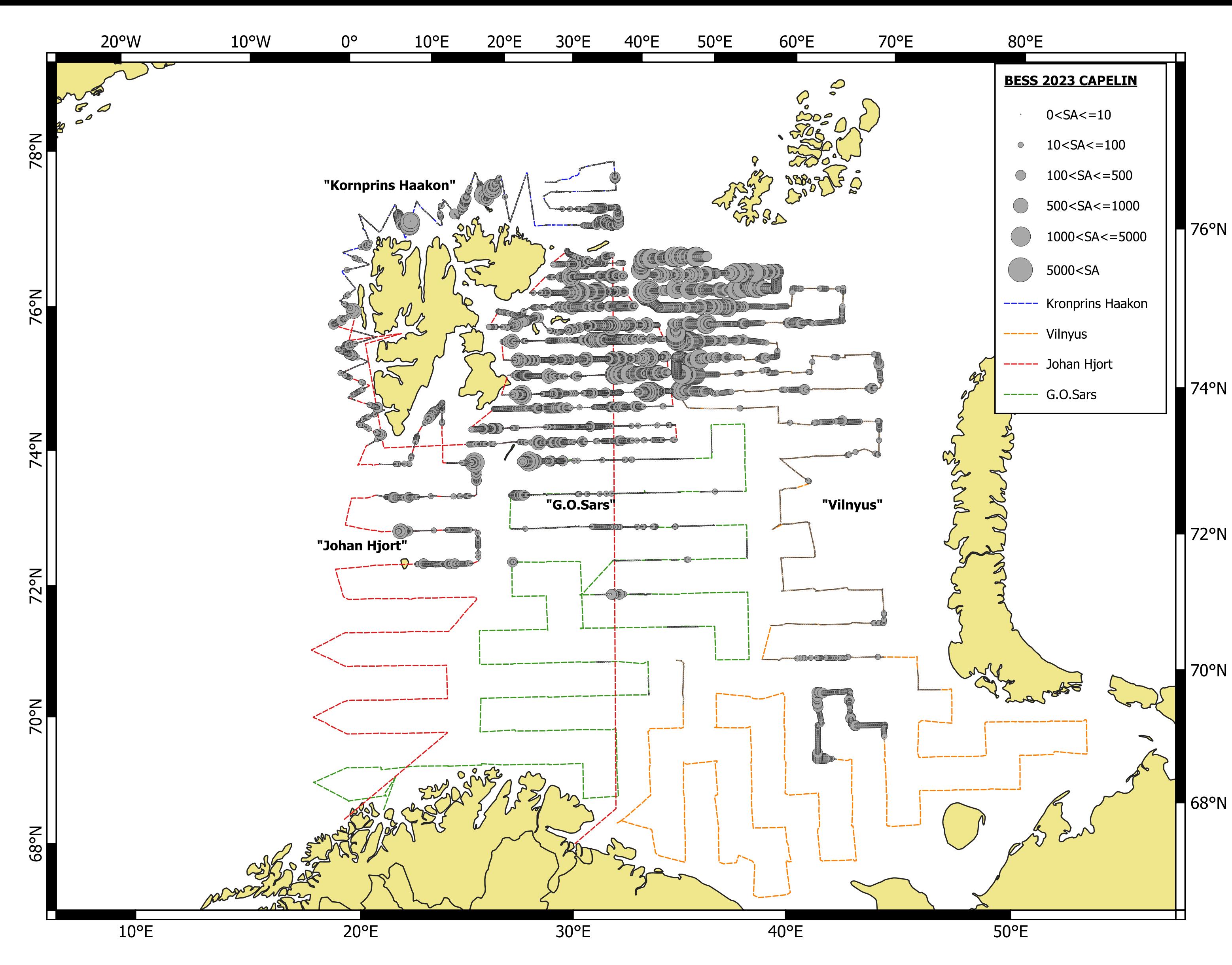
7.2 Polar cod (Boreogadus saida)
7.2.1 Geographical distribution
The acoustic recordings of polar cod are shown in Figure 7.2.1.1. The concentrations east of the Great Bank dominated, but there were also significant recordings on the westside of the Great Bank and northwest of Kvitøya. A spot with high polar cod concentrations was also recorded near the Kara Strait. It is very likely that some of the polar cod were distributed further to the north and northeast outside of the survey area. Thus, the polar cod estimate must be considered an underestimate of the population.
Figure 7.2.1.1 Geographical distribution of polar cod in autumn 2023 based on acoustic data. Circle sizes correspond to NASC values (m2/nmi2) per nautical mile.
7.2.2. Abundance estimation
The stock abundance estimates by age, number and weight in 2023 is given in Table 7.2.2.1 and the time series of abundance estimates are summarized in Table 7.2.2.2. The estimated means are from 1000 bootstrap replicas made in StoX 3.6.
The total estimated biomass of polar cod in 2023 is slightly below the long-term mean and less than 40% of the biomass estimated in 2021. All age groups from 1 to 4 were quite well represented in the population, with 1-year-olds being most abundant. 3-year-olds (2020 year-class) dominated in biomass, while there was a significant contribution in biomass also from 4-year-olds (2019-year class). The abundance of both these year classes were above the long-term average and they were observed as strong also in the 2021 survey. There was no polar cod estimation in 2022 due to poor survey coverage.
Table 7.2.2.1. Barents Sea polar cod. Summary of results from the acoustic estimate in August- October 2023. All values in the table are derived from average number and biomass at length and age from 1000 bootstrap runs in StoX 3.6.
Length (cm)
Age/year class
Sum (109)
Biomass (103 t)
Mean weight (g)
1
2
3
4
5
6
2022
2021
2020
2019
2018
2017
7-8
0.959
0.034
0.993
2.362
2.38
8-9
0.744
0.211
0.955
3.791
3.97
9-10
1.632
0.344
1.976
10.827
5.48
10-11
2.493
0.505
0.012
3.011
21.837
7.25
11-12
2.433
0.710
0.033
3.175
30.468
9.60
12-13
0.756
0.214
0.052
0.009
1.030
12.965
12.58
13-14
0.505
0.304
0.213
0.010
1.032
16.648
16.13
14-15
0.083
0.188
0.113
0.015
0.399
8.129
20.36
15-16
0.029
0.304
0.149
0.022
0.002
0.506
13.351
26.38
16-17
0.005
0.202
0.341
0.031
0.579
17.879
30.88
17-18
0.364
3.551
0.759
4.674
154.798
33.12
18-19
0.032
0.461
0.251
0.744
29.189
39.25
19-20
0.025
0.532
0.507
1.063
45.174
42.48
20-21
0.018
0.267
0.626
0.911
44.836
49.21
21-22
0.012
0.392
0.261
0.665
36.175
54.37
22-23
0.085
0.211
0.296
18.523
62.60
23-24
0.039
0.100
0.139
9.203
66.18
24-25
0.061
0.052
0.113
9.030
79.93
25-26
0.050
0.015
0.064
4.992
77.48
26-27
0.001
0.001
0.160
108.22
27-28
0.000
0.000
0.023
115.00
TSN (109)
9.640
3.465
6.240
2.912
0.070
0.000
22.328
TSB (103 t)
75.890
54.869
221.876
132.218
5.484
0.023
490.360
Mean length (cm)
10.497
12.81
17.85
19.72
24.48
27.50
15.46
Mean weight (g)
7.872
15.83
35.56
45.40
78.39
115.00
21.96
Estimates based on Target strength (TS) Length (L) relationship: TS= 21.8 log (L) – 72.7
Table 7.2.2.2. Barents Sea polar cod. Summary of acoustic estimates by age in August-October 2023. TSN and TSB are total stock numbers (109) and total stock biomass (103 tons) respectively.
Year
Age 1
Age 2
Age 3
Age 4+
Total
TSN
TSB
TSN
TSB
TSN
TSB
TSN
TSB
TSN
TSB
1986
24.038
169.6
6.263
104.3
1.058
31.5
0.082
3.4
31.441
308.8
1987
15.041
125.1
10.142
184.2
3.111
72.2
0.039
1.2
28.333
382.8
1988
4.314
37.1
1.469
27.1
0.727
20.1
0.052
1.7
6.562
86.0
1989
13.540
154.9
1.777
41.7
0.236
8.6
0.060
2.6
15.613
207.8
1990
3.834
39.3
2.221
56.8
0.650
25.3
0.094
6.9
6.799
127.3
1991
23.670
214.2
4.159
93.8
1.922
67.0
0.152
6.4
29.903
381.5
1992
22.902
194.4
13.992
376.5
0.832
20.9
0.064
2.9
37.790
594.9
1993
16.269
131.6
18.919
367.1
2.965
103.3
0.147
7.7
38.300
609.7
1994
27.466
189.7
9.297
161.0
5.044
154.0
0.790
35.8
42.597
540.5
1995
30.697
249.6
6.493
127.8
1.610
41.0
0.175
7.9
38.975
426.2
1996
19.438
144.9
10.056
230.6
3.287
103.1
0.212
8.0
33.012
487.4
1997
15.848
136.7
7.755
124.5
3.139
86.4
0.992
39.3
28.012
400.7
1998
89.947
505.5
7.634
174.5
3.965
119.3
0.598
23.0
102.435
839.5
1999
59.434
399.6
22.760
426.0
8.803
286.8
0.435
25.9
91.463
1141.9
2000
33.825
269.4
19.999
432.4
14.598
597.6
0.840
48.4
69.262
1347.8
2001
77.144
709.0
15.694
434.5
12.499
589.3
2.271
132.1
107.713
1869.6
2002
8.431
56.8
34.824
875.9
6.350
282.2
2.322
143.2
52.218
1377.2
2003*
32.804
242.7
3.255
59.9
15.374
481.2
1.739
87.6
53.172
871.4
2004
99.404
627.1
22.777
404.9
2.627
82.2
0.510
32.7
125.319
1143.8
2005
71.675
626.6
57.053
1028.2
3.703
120.2
0.407
28.3
132.859
1803.0
2006
16.190
180.8
45.063
1277.4
12.083
445.9
0.698
37.2
74.033
1941.2
2007
29.483
321.2
25.778
743.4
3.230
145.8
0.315
19.8
58.807
1230.1
2008
41.693
421.8
18.114
522.0
5.905
247.8
0.415
27.8
66.127
1219.4
2009
13.276
100.2
22.213
492.5
8.265
280.0
0.336
16.6
44.090
889.3
2010
27.285
234.2
18.257
543.1
12.982
594.6
1.253
58.6
59.777
1430.5
2011
34.460
282.3
14.455
304.4
4.728
237.1
0.514
36.7
54.158
860.5
2012
13.521
113.6
4.696
104.3
2.121
93.0
0.119
8.0
20.457
318.9
2013
2.216
18.1
4.317
102.2
5.243
210.3
0.180
9.9
11.956
340.5
2014
0.687
6.5
4.439
110.0
3.196
121.0
0.080
5.3
8.402
243.2
2015
10.866
97.1
1.995
45.1
0.167
5.3
0.008
0.5
13.036
148.0
2016
95.919
792.7
6.380
139.1
0.207
6.9
0.023
0.7
102.529
939.4
2017
13.810
121.8
8.269
200.8
1.112
34.3
0.003
0.1
23.195
357.1
2018**
1.900
16.4
0.980
23.1
0.240
9.4
0.014
0.6
3.124
49.6
2019**
6.109
49.8
1.217
30.3
0.214
6.3
0.014
0.8
7.555
87.2
2020
115.139
988.3
20.133
386.8
8.217
299.3
0.647
42.8
144.171
1720.8
2021
45.340
375.5
44.020
819.9
2.190
90.4
0.210
13.3
91.760
1299.0
2022
No data
2023
9.640
75.9
3.465
54.9
6.240
221.9
2.983
137.7
22.328
490.4
Average
31.550
254.6
14.060
314.4
4.560
171.4
0.530
28.7
50.740
770.6
* numbers partly based on VPA estimates
** incomplete survey coverage
7.3 Herring (Clupea harengus)
7.3.1 Geographical distribution
The main distribution of young Norwegian spring spawning herring (NSSH) was in the south-east (Figure 7.3.1.1). In addition, there were concentrations of young herring in the Central Bank area and the south-west.
Figure 7.3.1.1 Geographical distribution of herring in autumn 2023 based on acoustic recordings. Circle sizes correspond to NASC values (m2/nmi2) per nautical mile.
7.3.2 Abundance estimation
The estimated total number and biomass of NSSH in the Barents Sea in the autumn 2023 is shown in Table 7.3.2.1, and the time series of abundance estimates is summarized in Table 7.3.2.2. Total numbers in 2023 was estimated at ca. 104·109 individuals (Table 7.3.2.1). This is four times above the long-term average (Table 7.3.2.2). Abundance of all age groups 1-4+ were above the long-term average. In particular, the 1 and 2-year-olds were abundant. 1-year-olds are dominating in abundance while 2-year-olds are dominating the biomass estimate (Table 7.3.2.1). The abundance of both 1-year-olds and 2-year-olds were the second highest on record. While the high abundance of 1-year-olds follows from a year of very high 0-group abundance in 2022, the high abundance of 2-year-olds and relatively high abundance of 3-year-olds was not expected from previous BESS surveys. However, it should be noted that last year the eastern area was covered late and not included in the estimate.
Table 7.3.2.1. NSSH. Acoustic estimate in the Barents Sea in August-October 2023. All values in the table are derived from average number and biomass at length and age from 1000 bootstrap runs in StoX 3.6.
Length (cm)
Age/year class
Sum
(109)
Biomass
(103 t)
Mean
weight (g)
1
2
3
4
5
6
7
8
9
10
11
2022
2021
2020
2019
2018
2017
2016
2015
2014
2013
2012
7-8
0.683
0.683
1.367
2.00
8-9
0.450
0.450
1.487
3.31
9-10
3.030
3.030
15.056
4.97
10-11
2.793
2.793
20.823
7.45
11-12
5.683
5.683
56.132
9.88
12-13
13.582
13.582
171.034
12.59
13-14
20.162
20.162
297.378
14.75
14-15
12.880
0.184
13.063
232.500
17.80
15-16
2.767
1.134
3.901
87.321
22.38
16-17
1.103
3.611
4.714
129.007
27.37
17-18
0.499
6.621
7.120
235.625
33.09
18-19
0.193
8.433
8.626
345.932
40.10
19-20
0.121
4.118
4.239
206.942
48.81
20-21
0.151
2.926
3.077
187.537
60.95
21-22
0.017
3.307
0.049
3.374
229.971
68.17
22-23
0.489
0.489
36.000
73.57
23-24
0.499
0.071
0.570
54.251
95.23
24-25
0.931
0.977
1.908
201.204
105.45
25-26
0.524
2.311
2.835
337.016
118.89
26-27
0.626
0.071
0.697
98.565
141.45
27-28
0.141
0.394
0.536
91.284
170.46
28-29
0.002
0.005
0.007
1.470
208.05
29-30
0.002
0.003
0.002
0.008
1.421
182.57
30-31
0.007
0.008
0.007
0.022
5.201
231.47
31-32
0.029
0.010
0.040
10.505
264.18
32-33
0.345
0.164
0.250
0.759
219.956
289.65
33-34
0.125
0.194
0.011
0.330
104.838
317.41
34-35
0.032
0.479
0.032
0.053
0.596
195.126
327.51
35-36
0.255
0.227
0.160
0.641
208.015
324.44
TSN (109)
64.115
32.920
4.443
0.071
0.386
0.330
1.188
0.237
0.032
0.053
0.160
103.935
TSB (103 t)
925.193
1558.093
546.748
9.983
110.224
99.714
376.327
76.928
10.581
17.297
51.874
3782.962
Mean length (cm)
13.11
19.01
25.54
26.50
32.36
33.01
34.10
35.41
34.50
34.50
35.50
17.427
Mean weight (g)
14.43
47.33
123.07
141.45
285.62
301.84
316.68
324.12
327.51
327.51
324.44
36.40
Estimates based on Target strength (TS) Length (L) relationship: TS= 20.0 log (L) – 71.9
Table 7.3.2.2. NSSH. Summary of acoustic estimates of herring by age in autumn 1999-2023. TSN and TSB are total stock numbers (109) and total stock biomass (103 tons) respectively.
Year
Age 1
Age 2
Age 3
Age 4+
Total
TSN
TSB
TSN
TSB
TSN
TSB
TSN
TSB
TSN
TSB
1999
48.759
716.0
0.986
31.0
0.051
2.0
49.795
749.0
2000
14.731
383.0
11.499
560.0
26.230
943.0
2001
0.525
12.0
10.544
604.0
1.714
160.0
12.783
776.0
2002
No data
2003
99.786
3090.0
4.336
220.0
2.476
326.0
106.597
3636.0
2004
14.265
406.0
36.495
2725.0
0.901
107.0
51.717
3252.0
2005
46.380
984.0
16.167
1055.0
6.973
795.0
69.520
2833.0
2006
1.618
34.0
5.535
398.0
1.620
211.0
8.773
643.0
2007
3.941
148.0
2.595
218.0
6.378
810.0
0.250
46.0
13.164
1221.0
2008
0.030
1.0
1.626
77.0
3.987*
287*
3.223*
373*
8.866*
738*
2009
1.538
48.0
0.433
52.0
1.807
287.0
1.686
393.0
5.577
815.0
2010
1.047
35.0
0.315
34.0
0.234
37.0
0.428
104.0
2.025
207.0
2011
0.095
3.0
1.504
106.0
0.006
1.0
1.605
109.0
2012
2.031
36.0
1.078
66.0
1.285
195.0
4.394
296.0
2013
7.657
202.0
5.029
322.0
0.092
13.0
0.057
9.0
12.835
546.0
2014
4.188
62.0
1.822
126.0
6.825
842.0
0.162
25.0
13.011
1058.0
2015
1.183
6.0
9.023
530.0
3.214
285.0
0.149
24.0
13.569
845.0
2016
7.760
131.0
1.573
126.0
3.089
389.0
0.029
6.0
12.452
652.0
2017
34.950
820.0
2.138
141.0
3.465
412.0
0.982
210.0
41.537
1583.0
2018
No data
2019
13.650
172.0
0.209
15.1
6.000
756.0
1.600
487.0
21.460
1430.0
2020
0.231
13.0
1.816
189.0
11.59*
2796*
13.636*
2998*
2021
1.410
80.8
0.120
10.1
0.360
39.5
0.720
144.7
2.610
275.1
2022**
4.442
155.2
0.882
76.6
0.000
0.0
1.459
412.3
6.783
645.7
2023
64.115
925.2
32.920
1558.1
4.443
546.7
2.458
752.9
103.935
3783.0
Average
17.000
384.1
6.390
394.1
2.580
304.1
1.770
413.1
26.210
1305.8
*in mix with Kanin herring in the south-eastern part of the coverage area
**survey coverage only on Norwegian (western) side
7.4 Blue whiting (Micromesistius poutassou)
7.4.1 Geographical distribution
Blue whiting contributes to the mid-trophic pelagic component in the south-western part of the Barents Sea ecosystem. The Barents Sea is on the border of the distribution area for the blue whiting, but with incoming strong year-classes, increased abundance of young blue whiting in the Barents Sea is normally observed. The distribution of blue whiting from the BESS 2023 is shown in Figure 7.4.1.1. The distribution follows the shelf edge north to Svalbard/Spitsbergen and some low recordings were even found north of Svalbard/Spitsbergen.
Figure 7.4.1.1. Geographical distribution of blue whiting in autumn 2023 based on acoustic recordings. Circle sizes correspond to NASC values (m2/nmi2) per nautical mile.
7.4.2 Abundance by size and age
The estimated total number and biomass of blue whiting in the Barents Sea in the autumn 2023 is shown in Table 7.4.2.1, and the time series of abundance estimates is summarized in Table 7.4.2.2.
From 2004-2007 estimated biomass of blue whiting in the Barents Sea was between 200 000 and 350 000 tons (Table 7.4.2.2). In 2008 the estimated biomass dropped abruptly to only about 18% of the estimated biomass in the previous year, and it stayed low until 2012. From 2012 onwards it was variable, but the last six years it has been quite stable at a lower-than-average level despite that recruitment (abundance at age 1) in both 2021 and 2022 were high. This year estimated biomass was similar to the estimate from last year (Table 7.4.2.3).
The 2020 year class (3-year olds) dominated in both abundance and biomass, but all age groups are below average in abundance (Table 7.4.2.2).
Table 7.4.2.1. Blue whiting. Acoustic estimate in the Barents Sea in August-October 2023. All values in the table are derived from average number and biomass at length and age from 1000 bootstrap runs in StoX 3.6.
Length (cm)
Age/year class
Sum (106)
Biomass (103 t)
Mean weight (g)
1
2
3
4
5
6
7
8
9
10
11
12
13
14
2022
2021
2020
2019
2018
2017
2016
2015
2014
2013
2012
2011
2010
2009
18-19
0.2
0.2
0.0
33.69
19-20
0.7
0.1
0.8
0.0
36.12
20-21
3.6
1.6
5.2
0.2
42.58
21-22
12.3
4.1
16.5
0.8
49.78
22-23
6.9
0.7
5.3
12.8
0.8
59.51
23-24
1.4
10.8
6.1
18.3
1.3
71.64
24-25
4.2
13.9
3.6
21.7
1.8
84.09
25-26
16.3
12.3
1.8
30.4
3.0
97.47
26-27
9.5
12.0
7.9
29.5
3.3
111.33
27-28
4.3
18.6
8.4
7.5
0.7
0.3
39.8
5.1
126.99
28-29
14.9
6.7
1.8
0.8
6.1
30.3
4.3
141.73
29-30
7.7
2.9
5.4
1.0
0.7
1.3
19.1
3.0
158.65
30-31
3.2
1.8
1.4
2.3
0.1
0.5
0.9
0.2
10.4
1.8
169.02
31-32
1.5
1.2
2.8
1.4
1.2
8.2
1.5
185.80
32-33
0.2
1.6
2.5
1.4
2.2
0.6
8.5
1.8
207.61
33-34
0.4
1.1
3.1
4.3
0.7
9.6
2.2
226.45
34-35
0.4
1.0
0.6
5.4
0.6
7.9
2.0
255.50
35-36
0.8
0.5
1.1
0.4
1.0
0.0
0.1
3.8
1.0
274.15
36-37
0.3
0.4
0.4
0.1
1.2
0.3
302.89
37-38
0.1
0.1
0.1
0.1
0.3
0.1
362.40
38-39
0.2
0.1
0.3
0.1
305.66
39-40
0.0
0.0
0.0
326.00
TSN (106)
29.3
61.3
84.0
31.8
20.7
10.9
13.7
10.6
10.7
0.1
0.2
0.4
1.1
0.1
274.8
TSB (103 t)
1.7
5.4
9.9
4.3
3.3
2.1
2.5
2.4
2.3
0.0
0.0
0.1
0.3
0.0
34.5
Mean length (cm)
22.07
24.77
26.82
28.06
29.52
31.66
30.88
33.19
32.92
37.50
31.59
36.50
34.63
37.95
27.61
Mean weight (g)
56.73
88.93
117.61
135.55
159.36
194.21
183.46
226.21
218.64
362.40
191.84
302.89
253.66
354.19
125.37
Estimates based on Target strength (TS) Length (L) relationship: TS=20 log (L) - 65.2
Table 7.4.2.2 Blue whiting. Acoustic estimates by age in autumn 2004-2023. TSN and TSB are total stock numbers (106) and total stock biomass (103 tons).
Year
Age 1
Age 2
Age 3
Age 4+
Total
TSN
TSB
TSN
TSB
TSN
TSB
TSN
TSB
TSN
TSB
2004
669
26
439
33
1056
98
1211
159
3575
327
2005
649
20
523
36
1051
86
809
102
3039
244
2006
47
2
478
34
730
70
922
129
2177
235
2007
+
+
116
11
892
92
743
107
1757
210
2008
+
+
+
+
10
1
238
36
247
37
2009
1
+
+
+
6
1
359
637
366
65
2010
2
5
1
155
31
163
33
2011
2
+
2
+
13
2
93
22
109
25
2012
583
27
64
8
58
9
321
77
1025
121
2013
1
349
28
135
13
175
42
664
84
2014
111
5
19
2
185
20
127
28
443
55
2015
1768
71
340
29
134
15
286
44
2529
159
2016
277
13
1224
82
588
48
216
36
2351
188
2017
43
2
253
22
503
49
269
38
1143
115
2018
18
1
74
8
215
29
332
40
2019
54
2
64
5
66
8
162
27
347
43
2020
110
5
19
2
11
1
56
11
196
18
2021
406
17
58
5
39
5
67
13
584
40
2022
195
8
143
12
41
4
58
10
437
34
2023
29
2
61
5
84
10
100
17
275
34
Average
309
15
232
20
284
27
329
80
1088
105
Estimates based on Target strength (TS) Length (L) relationship: TS = 20 log (L) - 65.2 (Recalculation by Åge Høines, IMR 2017)
Note:«+» <0.5
Table 7.4.2.3 Summary of stock size estimates for blue whiting in 2022-2023. A comparison between the estimates this year and last year (yellow background).
Year class
Age
Numbers (106)
Mean weight (g)
Biomass (103 t)
2022
2021
1
29.3
194.6
56.52
40.13
1.7
7.8
2021
2020
2
61.3
143.2
88.57
86.31
5.4
12.4
2020
2019
3
84.0
40.7
118.40
103.31
9.9
4.2
2019
2018
4+
100.2
58.4
136.44
169.04
17.4
9.6
Total stock in:
2023
2022
Total
274.8
436.9
125.37
78.38
34.5
34.2
8 - Commercial Demersal Fish
This chapter is published in
Survey report (Part 2) from the joint Norwegian/Russian Ecosystem Survey in the Barents Sea and the adjacent waters August-October 2023
9 - Fish Biodiversity
Author(s):
Elena Eriksen
(IMR), Tatiana Prokhorova (VNIRO-PINRO), Andrey Dolgov (VNIRO-PINRO) and Dmitry Prozorkevich (VNIRO-PINRO)
9.1 Small non-target fish species
By E. Eriksen, T. Prokhorova, D. Prozorkevic and A. Dolgov
Figures by E. Eriksen
Despite the distribution and biology of the non-commercial fish species and their role in the Barents Sea ecosystem being investigated since mid-1990s (e.g. Dolgov, 1995; Wienerrother et al., 2011; Wienerrother et al., 2013 etc), their distribution patterns, abundance and biomass are still poorly studied. Since 2012 abundance and biomass of pelagically distributed juveniles of fish species from the families Agonidae, Ammodytidae, Cottidae, Liparidae, Myctophidae and Stichaeidae (called “small fishes” here) were calculated and presented in the Survey report (Figure 9.1.1). Calculation of the abundance and biomass was done using the same method as the calculation of the abundance of the 0-group of commercial species described in Chapter 6. The same polygons were used (Figure 6.2).
Figure 9.1.1. Total biomass of small non-commercial fishes in the Barents Sea in 1990-2023
In 2023, the total biomass of small fishes (9 317 tonnes for all these families) was higher than in 2021-2022 (Table 9.1.1). Total biomass of small non-commercial fishes was dominated by species from families Ammodytidae and Stichaeidae. Long term mean (LTM) for the period 1990-2023 is also presented. Time series for abundance and biomass indices calculated in SAS (1990-2003) and in R (2004-2023).
Composition of small fish biomasses varied between areas, the south-eastern and south-western polygons dominated by Ammodytidae, the northern and central polygons dominated by Stichaeidae and Liparidae.
Table 9.1.1. Abundance indices (AIc, in million individuals) and biomass (B, in tonnes) of pelagic juveniles of species from families Agonidae, Ammodytidae, Liparidae, Cottidae, Myctophidae and Stichaeidae in 1990-2023.
Year
Agonidae
Ammodytidae
Cottidae
Liparidae
Myctophidae
Stichaeidae
Total biomass, tonnes
AIc
B
AIc
B
AIc
B
AIc
B
AIc
B
AIc
B
1990
37
11
2099
1050
195
58
0
0
40
18
830
415
1552
1991
179
54
1733
866
2799
840
404
141
6
3
1565
783
2686
1992
85
25
1367
683
230
69
36
12
293
132
456
228
1150
1993
10
3
3425
1712
71
21
15
5
1536
691
0
0
2433
1994
808
242
33168
16584
3992
1198
11
4
13
6
0
0
18034
1995
39
12
4562
2281
93
28
2
1
40
18
3
2
2341
1996
117
35
7791
3895
310
93
35
12
274
123
0
0
4159
1997
32
9
3393
1697
282
85
184
65
12
5
1591
796
2656
1998
112
33
471
236
289
87
99
35
14
6
805
403
799
1999
388
116
1630
815
2460
738
865
303
12
5
1062
531
2508
2000
336
101
8549
4274
887
266
464
163
219
98
2129
1065
5967
2001
75
23
1052
526
206
62
97
34
153
69
681
340
1053
2002
20
6
3259
1630
37
11
46
16
17
8
0
0
1670
2003
27
12
389
140
435
216
24
21
0
0
1592
851
1241
2004
255
80
114
221
446
191
311
1213
76
42
1199
584
2330
2005
344
102
13848
18336
1012
609
3630
7185
12
5
1240
762
26999
2006
432
119
22368
11879
924
600
5639
2697
0
0
4856
1969
17264
2007
308
86
4364
7472
583
282
3540
1297
1
1
1558
830
9968
2008
124
44
255
244
18
12
51
88
38
24
337
181
593
2009
479
71
10578
2734
3182
833
953
274
263
126
4951
2701
6739
2010
244
59
378
164
146
78
268
132
6
6
3904
1293
1733
2011
139
52
955
507
315
146
907
426
4
2
4532
3014
4148
2012
175
60
8742
4907
272
170
1270
849
0
0
9933
4202
10188
2013
8
2
2118
2869
54
32
37
18
0
0
187
73
2993
2014
30
9
787
447
11
6
13
7
0
0
1301
641
1110
2015
65
27
2291
3139
929
525
442
196
0
0
3899
1932
5819
2016
108
38
10850
4129
880
535
3255
942
0
0
2148
970
6614
2017
29
11
2805
6986
4
12
881
153
0
0
541
271
7433
2018
633
259
1449
579
2675
2174
4010
2124
0
0
1382
819
5955
2019
766
228
587
390
1465
624
891
263
0
0
5452
2168
3673
2020
762
227
1884
18264
328
142
7316
2578
0,3
0
757
563
21774
2021
99
20
409
293
27
16
842
282
0
0
920
427
1037
2022
19
7
21
54
109
58
19
7
0
0
325
184
311
2023
34
10
8138
7842
3
4
10
21
0
0
2849
1440
9317
LTM
227
Agonidae were represented by Atlantic poacher Leptagonus decagonus. L. decagonus was distributed mostly in the northern area (Figure 9.1.2). The estimated indices in 2023 showed that their total abundance (34 million ind.) and biomass (10 tonnes) was lower than long-term mean values (227 million ind. and 68 tonnes (Table 9.1.1).
Figure 9.1.2. Spatial distribution of Agonidae in August-September 2023.
Abundance and biomass of Agonidae were calculated in R for the period of 2003-2023 for 15 WGIBAR-polygons (Figure 9.1.2). The highest densities of Agonidae were found in the North East during 2004-2007, 2009, and 2011, in the Great Bank in the 2013, 2016-2017 and in 2021, in the Central Bank 2008, 2015, 2018-2020, and in the Svalbard South in 2023 (Figure 9.1.3).
Figure 9.1.3. Spatial distribution of mean Agonidae densities by polygons in August-September 2003-2023.
Ammodytidae were represented by sandeel Ammodytes marinus and were widely distributed in the Barents Sea (Figure 9.1.4). In 2023, estimated abundance and biomass was almost twice higher than the long-term mean (4927 million ind. and 3.7 thousand tonnes correspondently) and was 8 138 million individuals and 7.8 tonnes, respectively (Table 9.1.1).
Figure 9.1.4. Spatial distribution of Ammodytidae in August-September 2023.
Total abundance and biomass of Ammodytidae calculated in R for the period of 2003-2023 for 15 polygons (Figure 6.2.). The highest densities of Ammodytidae were found in the Pechora during 2003, 2005-07, 2009-16, 2021 and 2023, in the Thor Iversen Bank during 2004 and 2008, in the South West in 2022, and in the Svalbard South during 2016-18 and 2020 (Figure 9.1.5).
Figure 9.1.5. Spatial distribution of mean polygon densities of Ammodytidae in August-September 2003-2023.
Stichaeidae were represented by snakeblenny Lumpenus lampraetaeformis, daubed shanny Leptoclinus maculatus, and stout eelblenny Anisarchus medius (Figure 9.3.6). In 2023, Stichaeidae were observed in the two separated ares in the north west and in the south east. In 2023, total abundance (2 849 million ind.) and biomass (1.4 thousand tonnes) of Stichaeidae was highest since 2019 and was higher than the long-term mean values of 1 869 million ind. (abundance) and 900 tonnes (biomass) (Table 9.1.1).
Figure 9.1.6. Spatial distribution of Stichaeidae in August-September 2023.
Total abundance of Stichaeidae calculated in R for the period of 2003-2023 for 15 polygons (Figure 6.2.). The highest densities of Stichaeidae were found in the Svalbard North and Svalbard South during almost all years (Figure 9.1.6). Other polygons contributed to the total abundance in lesser degree. While in last decades higher densities were found in Pechora (2017, 2021), Fr. Victoria Trough (2021) and Southeastern basin in 2023 (Figure 9.1.7).
Figure 9.1.7. Spatial distribution of mean polygon densities of Stichaeidae in August-September 2003-2023.
Cottidae were mostly represented by shorthorn sculpin Myoxocephalus scorpius, bigeye sculpin Triglops nybelini, ribbed sculpin Triglops pingelii and moustache sculpin Triglops murrayi. In 2023, Cottidae were restricted to some few stations in the north west, and their distribution was smaller than previous years (Figure 9.1.8). Total abundance (3 million ind.) and biomass (4 tonnes) was very low and was more than 200 times lower than the long term mean values of 799 million ind. (abundance) and 336 tonnes (biomass) (Table 9.1.1).
Figure 9.1.8. Spatial distribution of Cottidae and Liparidae in August-September 2023.
Total abundance of Cottidae calculated in R for the period of 2003-2023 for the same 15 polygons (Figure 6.2). The highest densities of Cottidae were found in the Fr. Victoria Trough during almost all years, in the Svalbard North in 2003-2005 and 2008, and in the Great Bank in 2018-2019 (Figure 9.1.9). Other polygons contributed to the total abundance in lesser degree.
Figure 9.1.9. Spatial distribution of mean polygon densities of Cottidae in August-September 2003-2023.
Liparidae were represented by gelatinous snailfish Liparis fabricii and nebulous snailfish Liparis bathyarcticus. In 2023, Liparidae distributed east and north-east for Svalbard/Spitsbergen (Figure 9.1.8). In 2023, estimated abundance and biomass were 10 million ind. and 21 tonnes, respectively. That is lower than the long-term mean values (1142 million ind. and 673 tonnes) (Table 9.3.1).
Total abundance of Liparidae calculated in R for the period of 2003-2023 for the same 15 polygons (Figure 6.2). The highest densities of Liparidae were found in the Great bank in 2004-2005, 2007 and 2019, and in the Fr. Victoria Trough during almost all years (Figure 9.1.10). Other polygons contributed to the total abundance in lesser degree.
Figure 9.1.10. Spatial distribution of mean polygon densities of Liparidae in August-September 2003-2023.
The following subchapters is published in
Survey report (Part 2) from the joint Norwegian/Russian Ecosystem Survey in the Barents Sea and the adjacent waters August-October 2023
9.2 Small non-target fish species
9.3 Fish biodiversity in the demersal compartment
9.4 Zoogeographic groups
10 - Commercial Shellfish
Ch 10 Commercial Shellfish is published in
Survey report (Part 2) from the joint Norwegian/Russian Ecosystem Survey in the Barents Sea and the adjacent waters August-October 2023
11 - Benthic Invertebrate Community
Ch 11 Benthic Invertebrate Community is published in
Survey report (Part 2) from the joint Norwegian/Russian Ecosystem Survey in the Barents Sea and the adjacent waters August-October 2023
12 - Marine Mammals and Seabirds
Ch 12 Marine Mammals and Seabirds is published in
Survey report (Part 2) from the joint Norwegian/Russian Ecosystem Survey in the Barents Sea and the adjacent waters August-October 2023