Revisjon av norsk-russisk økosystemtokt i Barentshavet (BESS)
BESS-toktet i norsk sone, som det er i dag og med forslag til revisjon
Preface
An effort to streamline the survey activity at the Institute of Marine Research (IMR) was initiated by the IMR leadership in December 2022. The purpose of this exercise is to balance the costs of the total cruise effort with the allocated budget. One of the candidate cruises of this streamlining, is the Norwegian-Russian Barents Sea Ecosystem Survey (BESS), referred to as NOR-RUS ecosystem cruise in autumn in IMR monitoring strategy and data systems.
Terms of reference: “The BESS should be reduced in scope by differentiating data and sample collection (i.e. different components can be collected with different efforts in time and space) according to changes in the biota and the need for deliverables to advisory committees and research”.
This report describes the current status and revision of the Norwegian sector of the BESS survey. The results from this revision will be presented to the IMR leadership on 20th March 2023.
Summary
BESS led by the EcoTeam, is organised in 16 main disciplines with an expert coordinator (EC) for each discipline. EcoTeam initiated the revision by including the ECs in the planning phase. The revision was prepared by EcoTeam and the ECs together with other experts in this field.
Each discipline was evaluated to streamline the survey effort regarding the need for annual coverage, geographical coverage, density of stations and transects, and scope of sampling. The results were discussed with the EC’s scientific counterpart at PINRO when necessary. Also, relevant IMR research groups were involved in an overall assessment of how a reduction in monitoring will affect their disciplines and time series.
A reduction in survey coverage in time and space is impossible without seriously influencing the scientific output from the survey. This relates to the fact that the wide range of ecosystem components we gather distribute throughout the whole Barents Sea. Furthermore, in most cases these variables exhibit high year-to-year variation in abundance and/or other biological traits. However, there are some prospects for periodisation on a yearly basis of specific sampling methods. Such a periodisation is already implemented for organic contaminants (biota and sediments) and radioactive pollution (sampled every third year).
A significant reduction in geographical and temporal coverage of BESS will seriously limit the value of data for ecological and ecosystem studies.
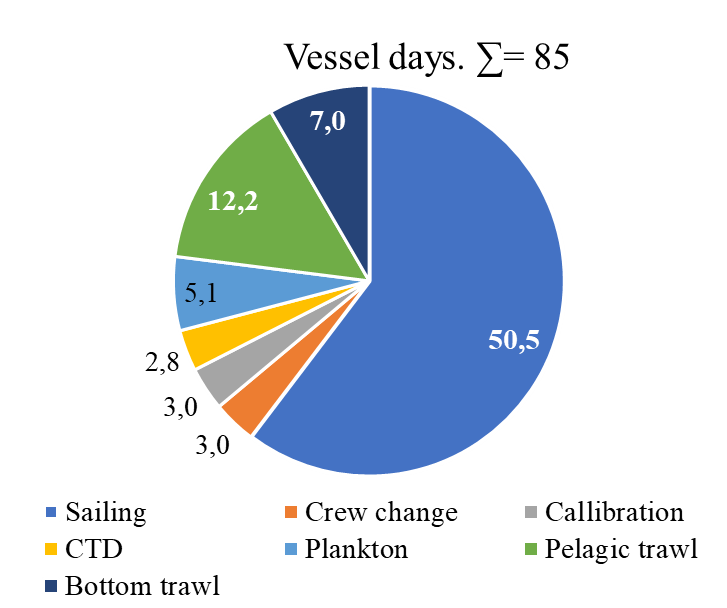
The results on the survey costs presented here are based on the design of BESS 2020. The costliest operation by the vessels is sailing, which takes half of the time allocated for BESS, not surprisingly to cover this large marine ecosystem of ca. 1 million km2.
Cost for taking one standard ecosystem station (CTD, plankton net WP2, pelagic and bottom trawls) will vary between vessels due to vessel costs. The cost of a standard ecosystem station will increase by 50-70 % when adding one equipment such as multinet or macroplankton trawls due to the extended station time. This happens even when the working time of that equipment is only about 30 minutes and is related to additional total station time. The cost of a standard ecosystem station will increase with 22 % when taking a Manta trawl (sampling microplastic). To reduce time spent at a standard station, both manta trawl and/or macroplankton trawls should be taken between standard stations to allocate time used for preparing and retrieving of the trawls to the sailing time.
Adding new activities, e.g. snow crab monitoring and new oceanographic sections, will add to the costs. However, the cost for extra oceanographic sections will be far less than if done by separate dedicated vessels.
Reducing sampling frequency to every third year will reduce statistical power, as well as the ability of detecting short-time fluctuations for groups/species. Ecosystem research on associations between top predators’ distributions, their prey and abiotic conditions, synoptic coverage of all ecosystem components by the BESS will be limited to each third years.
Mesozooplankton: Lack of vertical sampling of mesozooplankton by multinet at BESS-2 and BESS-3 implies no information on where in the water column the individuals are distributed. Such information is important for assessing of vertical overlap between the plankton and predators.
Macrozooplankton: Lack of sampling with macroplankton trawl at BESS-2 and BESS-3 implies no quantitative information on macrozooplankton species abundances and biomasses for the entire water column.
0-group fish: Lack of length measurement of 0–group fish limited to every second/third station will impact ecologically studies.
Expertise and skills of the scientists and technicians (species identification, routines) will be reduced if only practicing each third year.
The VNIRO-IMR cooperative work can be compromised if not kept in place on a regular basis.
1 - Revision of the Norwegian-Russian Barents Sea EcoSystem Survey (BESS)
An effort to streamline the survey activity at the Institute of Marine Research (IMR) was initiated by the IMR leadership in December 2022. The purpose of this exercise is to balance the costs of the total cruise effort with the allocated budget. One of the candidate cruises of this streamlining is the Norwegian-Russian Barents Sea Ecosystem Survey (BESS), referred to as NOR-RUS ecosystem cruise in autumn in IMR monitoring strategy and data systems.
Terms of reference: “The BESS should be reduced in scope by differentiating data and sample collection (i.e. different components can be collected with different efforts in time and space) according to changes in the biota and the need for deliverables to advisory committees and research”.
This report describes the current status and revision of the Norwegian sector of the BESS survey. The results from this revision will be presented to the IMR leadership on 20th March 2023.
2 - Historical development and earlier revisions
The need for an improved understanding of fluctuations of marine living resources for ecosystem-based management has been the driving force behind the increased survey effort. This has triggered the development of sampling and observation methodology, the design of state-of-the-art scientific research vessels, and the development of new technologies for processing a variety of sample-types.
It is important to realise that BESS originally was a result of an initiative to make the ecosystem monitoring in the Barents Sea more cost-effective. This was initiated by the need for more integrated surveys to provide relevant information about the whole ecosystem, and economic arguments related to better coordination of the monitoring. This resulted in the merging of five surveys conducted during late-summer-early autumn into one Barents Sea Ecosystem Survey (Eriksen et al. 20181). Since the start of BESS in 2004 (the effort in 2003 was restricted by lack of standard bottom trawl on Russian vessels), the survey has undergone numerous minor revisions and absorbed new and existing aspects of monitoring of the ecosystem including impacts of climate change and other anthropogenic pressures. The BESS also included standard oceanographic sections as part of the survey coverage to optimise IMRs costs. In addition, training of scientific personal onboard and dedicated courses (fish plankton, and benthos species identification) in the laboratory have raised competence level and data quality.
As a result of this development, BESS already represents a cost-effective and streamlined platform for a broad spectrum of ecosystem monitoring in the Barents Sea. It fulfils the IMR, national and international goals of development towards ecosystem-based advice and management, and represents an international gold-standard for survey-based ecosystem monitoring. It is also worth noting that BESS is continuously developing by assimilating new monitoring objectives, methodology, and technology with the aim of becoming even more cost-effective, while also improving the scientific potential.
3 - Objectives of BESS
The purpose of BESS is to: 1) Monitor the state of and changes in the Barents Sea ecosystem 2) obtain necessary data for stock advice and 3) gather relevant data for research.
The leading principles for BESS were discussed at the March meeting in 2016, where an agreement was reached, and the final decision was signed by the IMR and PINRO/VNIRO leaders. The leading principles for BESS are:
Full geographical coverage
Fixed periods
Synoptic stability
Stability in research vessels, with known capabilities, characteristics, and properties
Sampling conducted as synoptical as possible across vessels and between years
New sampling must not influence existing sampling while we are exploring new technologies
4 - Overview of the current status of BESS
BESS covers the entire Barents Sea to document the ocean climate, physical, chemical environment, and population status of plankton, benthic communities, fish, seabirds and marine mammals, their interactions, and human impacts, including pollution. In a typical year, the coverage of the Norwegian part of the survey takes 90 days, which constitutes close to 20% of the total IMR survey activity in the Barents Sea.
Over a hundred time series are used in stock assessment of commercial fish, and crustaceans, and assessment of ecosystem status provide valuable insight into interannual and long-term variations in the ecosystem. This is essential for assessing climate impacts on the various commercially and ecologically important stocks.
The BESS is a platform serving the entire IMR research community with necessary data collection, testing of new equipment, training of scientists and research technicians from different disciplines, and knowledge flows across the research programs and groups.
Since the initiation of BESS, more than 200 per-reviewed papers have been published in several high-ranking journals (Appendix III), and national and international reports providing management advice for sustainable harvesting of living marine resources (the Ministry of Industry, Trade and Fisheries), environmental status reporting (The Ministry of Climate and Environment), protection of marine areas and resources (Norwegian Management Plan), status and change in the Arctic Ocean (Arctic Council), and others. The BESS data are also used in several ICES working groups such as; AFWG, WGWIDE, WGEF, WGIBAR, WGRED, WGOH and NAFO/ICES Pandalus WG.
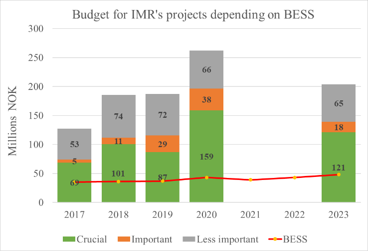
The BESS budget is, on a yearly basis, 4-6 times lower than the total budget for all the IMR projects it serves (Figure Ap.4). This clearly demonstrates the important (and for some projects essential) role of the BESS as a stable and secure investment into ongoing and future projects.
Details about the current status of BESS and the single components included in the survey are described in Appendix II and Appendix IV, respectively.
5 - Revision of BESS
BESS led by the EcoTeam is organised in 16 main disciplines with an expert coordinator (EC) for each discipline (Appendix I). EcoTeam initiated the revision by including the ECs in the planning phase. The revision was prepared by EcoTeam and the ECs together with other experts in this field.
Each discipline was evaluated to streamline the survey effort regarding the need for annual coverage, geographical coverage, density of stations and transects, and scope of sampling. The results were discussed with the EC’s scientific counterpart at PINRO when necessary. Also, relevant IMR research groups were involved in an overall assessment of how a reduction in monitoring will affect their disciplines and time series.
Most of the revision was performed qualitatively (expert evaluation) given the short time frame, but revision of the effect on sampling error of reduced biological sampling and coverage (geographical and temporal) was performed quantitatively . The revision process and analyses were guided by statisticians. Analyses and consequences of possible reduction in sampling effort for each discipline are presented in Appendix IV.
EcoTeam is responsible for providing the background for the evaluation and putting the feedback received from the different disciplines in a context of an ecosystem-based monitoring survey, at the same time aiming to preserve the ecosystem dimension of the survey.
Different alternatives to BESS based on the revision are presented.
5.1 - Assessment of survey effort
Here we summarise the ECs recommendations for possible reduction of sampling effort (geographical, temporal and a combination of these two). Table 1 presents the different disciplines and ecosystem components with proposed reduction of sampling effort. Components with a critical level of current sampling effort are indicated in red; components with potential reduction of sampling effort to some degree are indicated in orange (the reduction will influence the quality of estimators due to increase uncertainty) and less-influenced components in green (the reduction of sampling effort will not influence quality of estimators). Table 1 also shows different levels of deliverables (estimators uses for stock advice (dark blue) and for other purposes such as ecosystem or ecological studies (light blue).
As can be seen from table 5.1. and Appendix IV, a reduction in survey coverage in time and space is impossible without seriously influencing the scientific output from the survey. This relates to the fact that the wide range of ecosystem components we gather distribute throughout the whole Barents Sea. Furthermore, in most cases these variables exhibit high year-to-year variation in abundance and/or other biological traits. However, there are some prospects for periodisation on a yearly basis of specific sampling methods. Such a periodisation is already implemented for organic contaminants (biota and sediments) and radioactive pollution (sampled every third year).
Note that a significant reduction in geographical and temporal coverage of BESS also will seriously limit the value of data for ecological and ecosystem studies.
Investigations
Purpose
Equipment
Geographical (station density and area coverage)
Temporal (reducing frequency)
Combination time and space
Plankton: provide plankton biomass indices, obtain data for ecosystem studies including standing stock of plankton biomass and taxonomic abundance, available food for higher trophic levels, and climate effects
Multinet
Spatial sampling density - should be kept unchanged
Can be reduced to every second year for the whole Barents Sea
Can be reduced to every second year for the whole Barents Sea
WP2
Plankton indices - reduced spatial sampling density will reduce precision and accuracy of estimates - not acceptable
Plankton indices - increased uncertainty and reduced temporal resolution - consequences for ecosystem assessments and studies, hence, not acceptable (not considering the area north and west for Svalbard)
Plankton indices - increased uncertainty and reduced temporal resolution - consequences for ecosystem assessments and studies, hence, not acceptable (not considering the area north and west for Svalbard)
WP2
Geographical coverage west and north of Svalbard could be reduced to every second year.
Geographical coverage west and north of Svalbard could be reduced to every second year.
Geographical coverage west and north of Svalbard could be reduced to every second year.
Macroplankton trawl
Need to increase from ca. 5 to 10 trawls per year
Need to increase from ca. 5 to 10 trawls per year
Need to increase from ca. 5 to 10 trawls per year
Macroplankton: provide a biomass of krill, amphipods and jellyfish, obtain data for ecosystem studies (feeding conditions for kye species, food web, energy flow)
Pelagic trawl
Macroplankton indices - not acceptable
Macroplankton indices: no meaning with index
Macroplankton indices - not acceptable
For ecosystem studies only
For ecosystem studies only
For ecosystem studies only
0-gruppe fish investigations : 1. estimation of year class strength (11 species), 2. support capelin assessment (biol.data of older fish), and 3 ecosystem studies (as prey for fish, sea birds, marine mammals, as plankton consumer, energy flow…
Pelagic trawl
0-group fish indices: decrease trawl density may increase uncertainties. 10 stations on the continental slope could be excluded
0-group fish indices: no meaning with index
0-group fish indices: no meaning with index
Capelin assessment: to some degree
Capelin assessment: increased uncertainties for capelin age 1
Capelin assessment: not acceptable
For ecosystem studies only
For ecosystem studies only
For ecosystem studies only
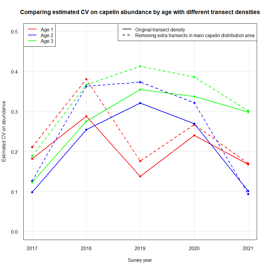
Pelagic fish : to provide an annual quota advice on capelin; potential young NSS-herring estimate as input to assessment; obtain data from the mid-trophic level which can be used for ecosystem studies
Pelagic trawl
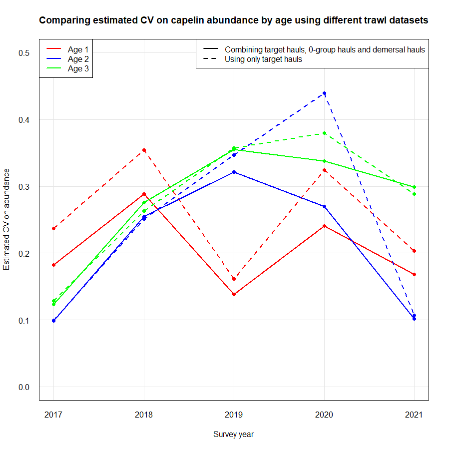
Similar coverage area and transect density as now, but including only target hauls (frequency of target hauls increased somewhat compared to presently since we now also rely on 0-group hauls)
Every second-year full ecosystem coverage, and every second year coverage of only the main capelin distribution area. The young herring and blue whiting area would then only be covered bi-annually
Annual coverage of only the main capelin distribution area with a transect density similar to what it is now and only target hauls carried out. The young herring and blue whiting would then not be covered
Demersal fish: provide input data for NEA cod and haddock assessments, obtain data for ecosystem studies
Bottom trawl
Exclude bottom trawls deeper than 400 m depth
Not acceptable due to the assessments of cod and haddock is done annually
Not acceptable due to the assessments of cod and haddock is done annually
Reduce coverage in the North-easternmost Barents Sea
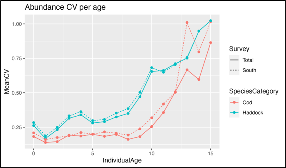
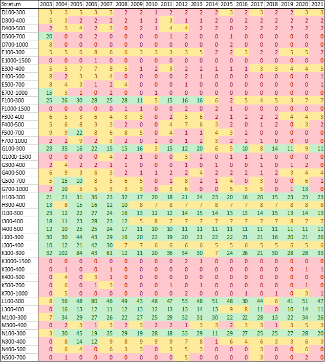
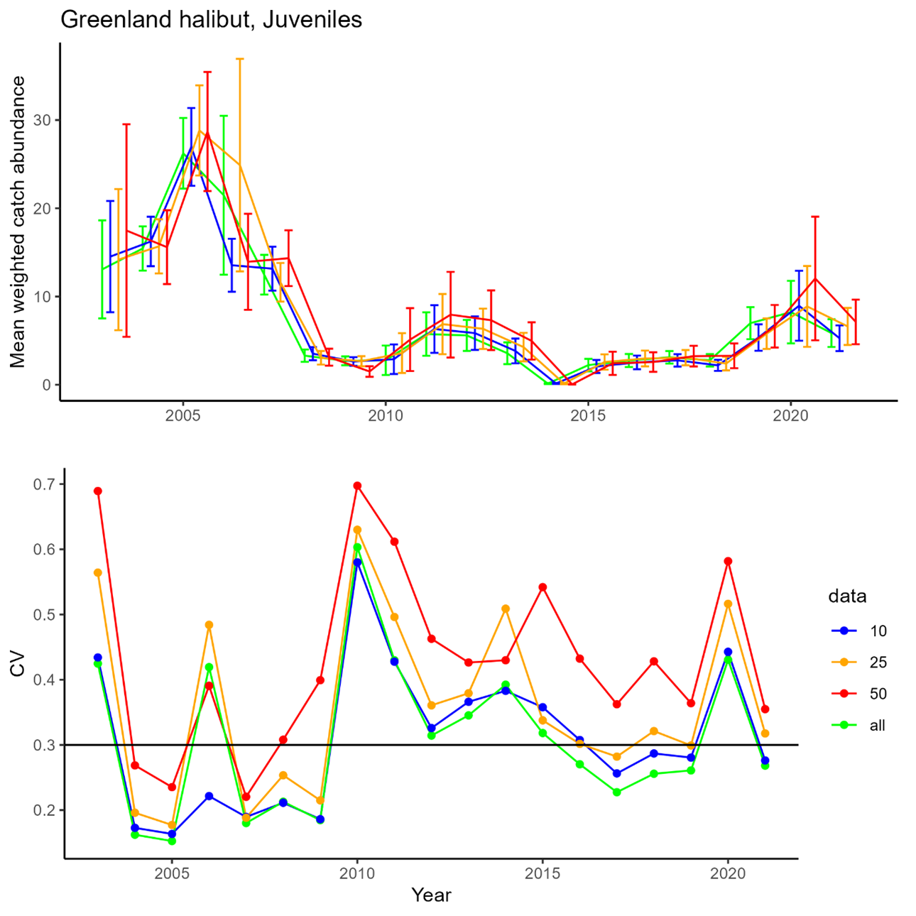
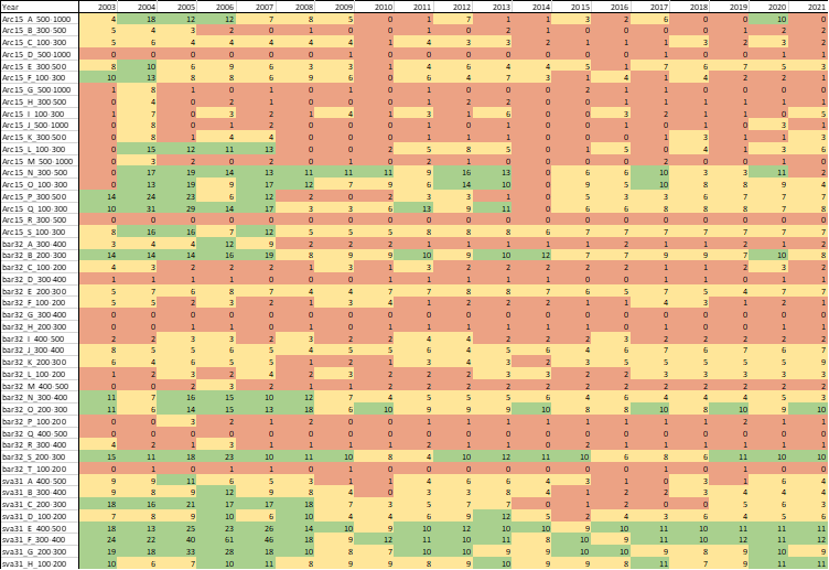
Deep water species and cartilaginous fish : 1. biomass and abundance indices for juvenile and adult Greenland halibut, beaked and golden redfish; 2. Biological information for these species
Bottom trawl
Greenland halibut (central and south): N_stations per stratum can go under critical level, but index might still be usable.
Greenland halibut (central and south): affect adult fish index, but it might still be useful
Greenland halibut (central and south): not acceptable
Greenland halibut (north) Not acceptable due to patch distribution of juveniles
Greenland halibut (north): Will potentially miss sporadic recruitment events.
Greenland halibut (north): not aceptable
Beaked redfish (south): increased uncertainties
Beaked redfish (south): increased uncertainties
Beaked redfish (south): not aceptable
Fish biodiversity : obtain data for fish biodiversity, population size and ecological studier (new vs species moving out of the area, distribution shift, food web)
Pelagic/Bottom trawl
Full geographical coverage is necessary to cover different habitats and thus species
Annual coverage is desirable, but a reduction might be acceptable as long as the whole area is covered at least every second year
Not acceptable
Crabs : to provide input data for the snow crab stock assessment (density, population structure, biological parameters) and ecological studies
Bottom trawl
Campelen trawl not representative for snow crab, demersal trawl coverage could be reduced outside of Storbanken/Sentralbanken area
Campelen trawl not representative for snow crab, demersal trawl coverage could be reduced outside of Storbanken/Sentralbanken area
Campelen trawl not representative for snow crab, demersal trawl coverage could be reduced outside of Storbanken/Sentralbanken area
Campelen trawl not suitable for snow crab sampling, new AUV/video sampling to be implemented
Campelen trawl not suitable for snow crab sampling, new AUV/video sampling to be implemented
Campelen trawl not suitable for snow crab sampling, new AUV/video sampling to be implemented
Shrimps : provide input data for the northern shrimp stock assessment, obtain data to ecological (population structure, natural mortality osv) and ecosystem (species interaction, climate impact osv) studies
Bottom trawl
Bottom trawl coverage (increased distance between tawl stations) could be reduced in northeast (north of Novaja Zemlja) and southwest Barents Sea (Tromsøflaket, Bear Island area)
Bottom trawl coverage outside Sentralbanken/Storbanken/Eastern Basin/Svalbard areas could be reduced to every other year
Bottom trawl coverage outside Sentralbanken/Storbanken/Eastern Basin/Svalbard areas could be reduced to every other year and lower station density
Bottom trawl coverage could be reduced (larger distance between tawl stations) outside Sentralbanken/Storbanken/Eastern Basin/Svalbard areas
Annual bottom trawl coverage of Sentralbanken/Storbanken/Eastern Basin/Svalbard areas is crucial for stock index
Annual bottom trawl coverage of Sentralbanken/Storbanken/Eastern Basin/Svalbard areas is crucial for stock index
Bottom trawl coverage of Sentralbanken/Storbanken/Eastern Basin/Svalbard areas is crucial for stock index
Benthos : temporal and spatial distribution and variation of benthos
Bottom trawl
Not acceptable
full coverage of the benthos identification each second year with 4 experts onboard ships covering areas with high species diversity and biomass
Not acceptable
Organic contaminants : collect samples for analyses of organic contaminants in marine biota
Trawls s
it is important to take samples in different areas
already reduced the sampling to each third year
Not acceptable
Radioactive pollution : collect samples for analyses of radioactive pollution in marine biota
CTD, grab, trawls
it is important to take samples in different areas
already reduced the sampling to each third year
Not acceptable
Radioactive pollution : collect samples for analyses of radioactive pollution near the sunken nuclear submarine “Komsomolets”
CTD, grab
Not acceptable
Could be be performed from other cruises in other years
Not evaluated
Table 5.1. Overview of consequences of sampling effort reduction
5.2 - Assessment of economic costs
EcoTeam evaluated the different cost sources for vessels used based on 2020, 2021 and 2022 BESS data. Vessels log files were used to identify start and stop times for each sample operation (operation time), which further were used to estimate the work time for each equipment (Figure 5.1). Start and stop of an ecosystem station (station time) was defined as the period between the vessel reached a speed <5 knots before arriving and obtaining a speed >5 knots when leaving a station.
CTD and WP2work time is considered equal to the operation time. For pelagic and bottom trawls, operation time indicates time when the fish are caught by the gear at a defined depth. For these trawl gears, the time taken for setting and heaving the trawl needed to be added to obtain proper working time. We therefore added 30 minutes extra to the operation time for trawls.
Positioning of the vessel, return to the station location after a finishing an operation, relocating crew between different equipment, and preparation of the equipment itself with related technical problems were difficult to link to specific equipment. The time used for these station specific operations for all equipment were estimated as the difference between station time and summed working time. This time was then divided equally between all operations at that station and added to each equipment work time to obtain total time use of each operation at an ecosystem station. Our estimation of time used per equipment is a crude approximation, based on data and knowledge.
Figure 5.1. Vessels log files were used to identify start and stop times for each sample operation (operation time), which further were used to estimate the work time for each equipment.
The time needed for sampling of different ecosystem components was related to the use of specific equipment. Time per equipment usually varied with area, depth, and weather condition, and it was evident that the time used for each operation increased when other operations were added to the station. The increase in station time when adding an operation is therefore not simply the additional working time of that operation.
The results on the survey costs presented here are based on the design of BESS 2020. The costliest operation by the vessels is sailing, which takes half of the time allocated for BESS, not surprisingly to cover this large marine ecosystem of ca. 1 million km2
The cost of standard ecosystem station (CTD, plankton net WP2, pelagic and bottom trawls) will vary between vessels due to vessel costs. The cost of a standard ecosystem station will increase by 50-70 % when adding one equipment such as multinet or macroplankton trawls due to the extended station time. This happens even when the working time of that equipment is only about 30 minutes and is related to additional total station time. The cost of a standard ecosystem station will increase with 22 % when taking a Manta trawl (sampling microplastic). To reduce time spent at a standard station, both manta trawl and/or macroplankton trawls should be taken between standard stations to allocate time used for preparing and retrieving of the trawls to the sailing time.
5.2.1 - Additional tasks for BESS
Oceanographic sections
Three standard oceanographic sections (Vardø-Nord extended, Hinlopen and Sørkapp-west) were incorporated into BESS in different periods for making the IMR monitoring program more cost-efficient. Cost for taking these sections during the BESS were estimated and thus could be easily added to BESS program. In total, 6.5 days are needed to take these three oceanographic sections, corresponding to a vessel cost of 1.4 million NOK. The cost for scientific personal (9-13 experts with approximately 15 thousand NOK per person per day) for these extra 6.5 days of survey will add 0.7-1.1 M NOK to this sum. The BESS generally ends in the north and therefore needs sailing time to harbour (Kirkenes or Tromsø). The vessel covering the northern area of BESS usually carries out the standard section Vardø-Nord extended during its southwards sailing at the end of the survey. This resulted in one and a half extra day of delay and increased budget for BESS. On the other hand, the coverage of these sections by BESS saves many days and millions of NOK for the IMR monitoring program, when compared to taking these sections with separate dedicated vessels.
Snow crab monitoring
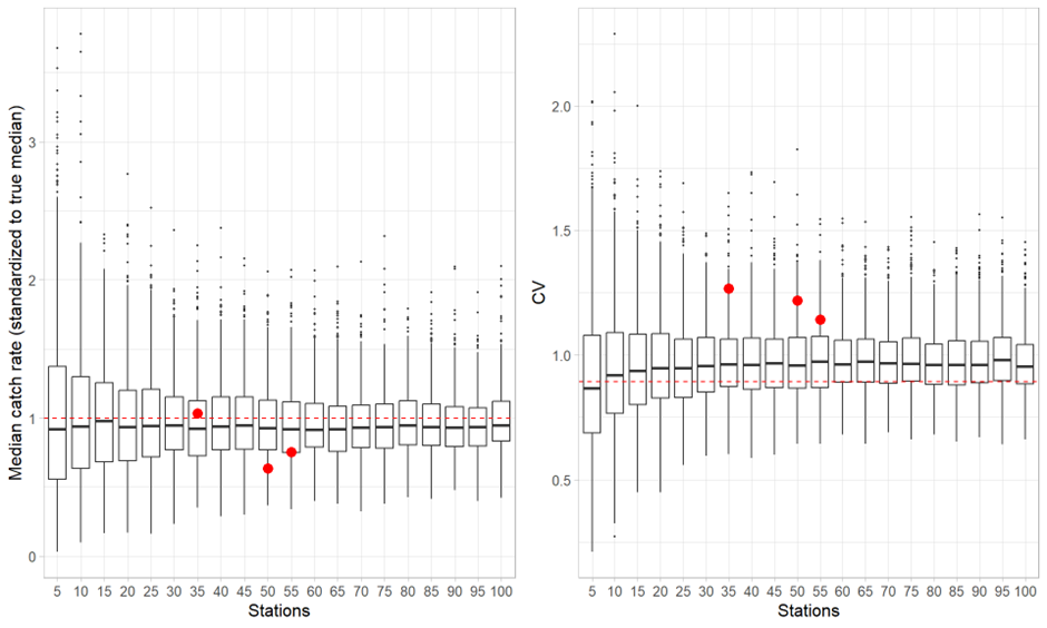
Standard investigation of snow crab during the ecosystem survey is not considered to be representative for abundance and demography of snow crab population in the Barents Sea. A simulation study resampling predicted snow crab distribution combined with video transect data indicated that at least a minimum of 30 to 40 transects are required in the snow crab fishing area for good estimates of their abundance. Furthermore, from the AUV we will get density data only, further limiting knowledge on sex, size composition, and other biological parameters. Implementation of AUV as a new method for surveying snow crab is under construction. To ensure adequate sampling effort from the AUV equivalent to the area coverage as we have today, at least 10 more ship-time days are required. At the same time as the AUV is sampling data, the time spent in the area will be used to sampling biological data with other equipment.
It will be difficult to do other surveys at the same time and thus it will have negative consequences for a synoptic coverage. Adding 10 extra days should be at the start of the survey period, and not at the end. This is due to that the time available between end of the survey and the Norwegian Russian Fisheries commission meeting is already very limited. Additional 10 days will cost 4.85 million (vessel 2.61 million NOK and manning 2,24 million NOK). Thus, the BESS need to be extended with 10 days with an additional budget increase of 4.85 million NOK.
5.3 - New options for the BESS
The main principle for suggesting alternatives of a new BESS was to obtain the observational data needed to provide research-based advice on vital stocks such as capelin, cod, haddock, Greenland halibut, redfish, crabs, and northern shrimps and maintaining long-term time series (as stated in the Purpose- and Mission letter at IMR). The new BESS approaches will still maintain deliverables to user-oriented products (advice and reports to different Ministries), research (models and articles), and capture main fluctuations in ecosystem with climate change.
Based on table 5.1 and appendix IV, the geographic extent is kept, except removal of some pelagic ecosystem stations along the continental shelf in the west. Some periodisation is possible and could be decided later. In addition, adjustments of onboard sampling are performed.
We evaluated three options for carrying out the BESS: BESS-1 full ecosystem surveys (approximately the same level as current BESS with some effectivization/improvement of the survey design (Figure 5.2)), BESS-2 reduced survey with pollution, and BESS-3 reduced survey without pollution. These three options of the BESS could be repeated with a certain periodicity and still maintain deliverables for research-based management/stock advice.
Figure 5.2. Improved BESS design for the Norwegian part of the Barents Sea.
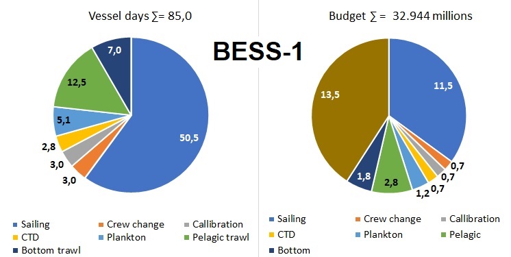
Figure 5.3. BESS_1 vessel days and budget
A full ecosystem survey ( BESS-1, figure 5.3 ) means maintaining full geographic coverage with slightly improved survey design, all ecosystem components (abiotic, biotic (from phyto-, meso, macrozooplankton, other invertebrates, benthos, fish and marine mammals), contaminants in the biota and sediments. Simultaneously collected data across the entire ecosystem increase the value of the data relevant for ecological and ecosystem studies, including response to ongoing climate changes and use in ecosystem models. In addition, it prolongs simultaneous time series data to enable process studies. In total 85 days are needed to carry out the BESS-1, including personnel, corresponding to 33 million NOK.
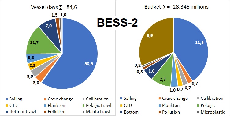
Figure 5.4 Bess-2 vessel days and budget
Reduced BESS with pollution ( BESS-2, figure 5.4) means maintaining full geographic coverage with some improvement of survey design compared to current BESS (Figure 5.4). Almost all components (except species identification for marine mammals and benthos) and including monitoring of pollution as organic contaminants (in biota and sediments), radioactive pollution and marine litter, including microplastic. Plankton sampling will be reduced to WP2 only. Pelagic stations (often called 0-group stations) in the southwest will be reduced with 10 stations and these will be replaced by acoustic transects covering the BS southernmost distribution of blue whiting. Length measurements of 0-group fish will be reduced to every second station and to key species only. Processing of commercially important demersal fish species will be kept at the same level, while non-commercial fish species will be limited to length measurements of 20-30 specimens per sample. Due to streamlining of the fish sample processing, manning in fish lab could be reduced from three to two persons per shift corresponding to a reduction from six to four on board J. Hjort and G.O. Sars covering southern and western areas. Reduction of manning only corresponds to 1.2 million NOK compared to BESS-1.
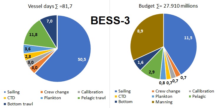
Figure 4. BESS-3 vessel days and budget
Reduced ecosystem survey ( BESS-3 ) means maintaining full geographic coverage and almost all components, except marine mammals and benthos species identification, radioactive pollution, and marine litter, including microplastics. Plankton sampling will be reduced to WP2. Pelagic stations (often called 0-group stations) in southwest will be reduced with 10 stations and they will be replaced by acoustic transect for covering the BS southmost distribution of blue whiting. Length measurements of 0-group fish will be reduced to every second station and to key species only. Processing of commercially important demersal fish species will be kept at same level, while non-commercial fish species will be limited to length measurements of 20- 30 specimens only. Due to streamlining of fish sample processing manning in fish lab could be reduced from three to two persons per shift corresponding to a reduction from six to four on board J. Hjort and G.O. Sars covering southern and western areas. Reduction of manning only corresponds to 1.2 million NOK compared to BESS-1.
The cost related to work on land for EcoTeam and ECs (ca 3.3 million), travel expenses for scientific staff participating at BESS and transport of samples (ca 0.7 M NOK) were not included in estimation of BESS-1, BESS-2 and BESS-3 costs. EcoTeam is responsible for planning, caring out and reporting the survey (approximately cost of 1 M NOK), while ECs are responsible for preparation and reporting of the results (approximately 2.3 M NOK) Thus, additional expenses (about 4 million) need to be taken into consideration for these three suggested options of the BESS.
Coverage of one or more oceanographic sections (Vardø-Nord extended, Hinlopen and Sørkapp-west) could be easily added to one or several BESS options. It will be cheaper for IMR monitoring to use BESS vessels which operates in the oceanographic section areas anyway, instead of using separate vessels covering the oceanographic sections. The cost for BESS should be increased respectively to the days and budgets (see above) needed for covering the oceanographic sections.
5.4 - Consequences of reducing the survey effort
5.4.1 - Reducing sampling frequency
Reducing sampling frequency to every third year will reduce statistical power, as well as the ability of detecting short-time fluctuations for groups/species. Ecosystem research on associations between top predators’ distributions, their prey and abiotic conditions, synoptic coverage of all ecosystem components by the BESS will be limited to each third years.
Mesozooplankton: Lack of vertical sampling of mesozooplankton by Multinet at BESS-2 and BESS-3 implies no information on where in the water column the individuals are distributed. Such information is important for assessment of vertical overlap between the plankton and predators.
Macrozooplankton: Lack of sampling with Macroplankton trawl at BESS-2 and BESS-3 implies no quantitative information on macrozooplankton species abundances and biomasses for the entire water column.
0-group fish: lack of length measurement of 0–group fish will be limited to every second/third station will impact ecologically studies.
Expertise and skills of the scientists and technicians (species identification, routines) will be reduced if only practicing each third years.
The VNIRO-IMR cooperative work can be compromised if not kept in place on a regular basis.
6 - Appendix I: Responsible participants
EcoTeam (5)
Elena Eriksen – project manager
Herdis Langøy Mørk – co-project manager and data manager
Geir Odd Johansen - responsible for planning and carrying out the survey
Gro I. van der Meeren - responsible for reporting and communication
Stine Karlson - responsible for arranging sampling and map production
Expert coordinators by discipline (16)
Physical and chemical oceanography – Randi Ingvaldsen
Pollution: Radioactivity - Hilde Elise Heldal
Pollution: Organic contaminants - Stepan Boitsov
Pollution: Marine litter and microplastics - Bjørn Einar Grøsvik
Mesozooplankton – Espen Bagøien
Macrozooplankton and 0-group fish - Elena Eriksen
Pelagic fish - Georg Skaret
Fish diversity - Rupert Wienerroither
Bottom fish - Edda Johannesen
Deep-water fish and cartilaginous fish - Kristin Windsland
Shrimps – Trude Thangstad
Crabs – Ann Merete Hjelset
Benthos – Anne Kari Sveistrup
Marine mammals – Nils Øien
Gear - Shale Pettit Rosen
Seafood parasites – Arne Levsen
7 - Appendix II: Current status of the Norwegian-Russian Barents Sea EcoSystem Survey (BESS)
This appendix provides an overview of how BESS is organised and conducted to achieve main objectives of the BESS and IMR. It presents the overall survey design of BESS, covering aspects like timing and survey progress, geographic coverage and ship tracks, how stations and transects are distributed, and the sampling methods and data retrieval for each main component of the survey. Also, the deliverables from the survey, its economic and scientific value, and development and innovation related to the survey are presented. BESS is a joint effort of IMR and PINRO-VNIRO. It is planned and decided in cooperation between Norwegian and Russian scientists, and secure comparable data collection from the entire Barents Sea used in joint assessment of commercial stocks and the ecosystem.
7.1 - Practical implementation, methodology and sampling
The need for more ecosystem knowledge, economic streamlining and better coordination of the monitoring resulted the merge of five surveys into one survey, BESS (Nakken et al. 2002, ref. in Eriksen et al. 2018). BESS started developing in 2004 and has gradually reached its current status through integrating more ecosystem components and anthropogenic pressures (Eriksen et al. 2018).
7.1.1 - Temporal structure
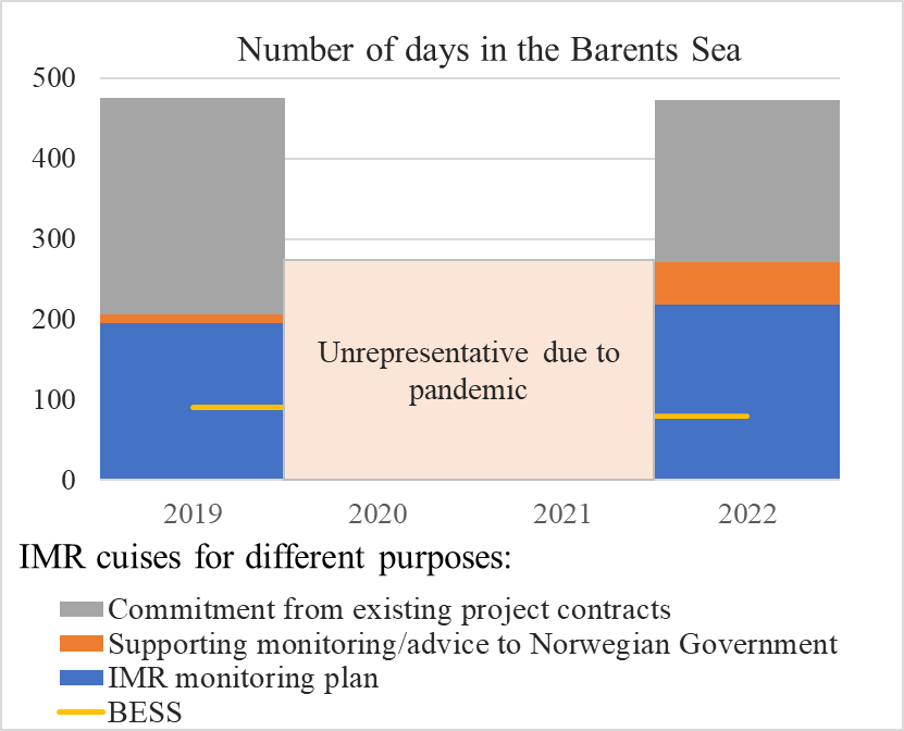
BESS is conducted in the period mid-August to early October every year with all components being sampled, except from organic and inorganic pollution which is sampled every third year. The total effort split on four vessels, 3 Norwegian and 1 Russian, are about 150 days, whereof 90 days are covered by Norwegian vessels. In a typical year the Norwegian part of the survey constitutes close to 20% of the total IMR cruise activity in the Barents Sea, and about 40 % of the activity listed in the IMR monitoring plan (Figure 7.1).
Figure 7.1. AII.1. Cruise activity at IMR in 2019 and 2022 in days, split on different priority categories. It is based on a combination of survey applications and survey plans and both IMR and rental vessels are included. The yellow line represents BESS activity.
7.1.2 - Geographic area and vessel track lines
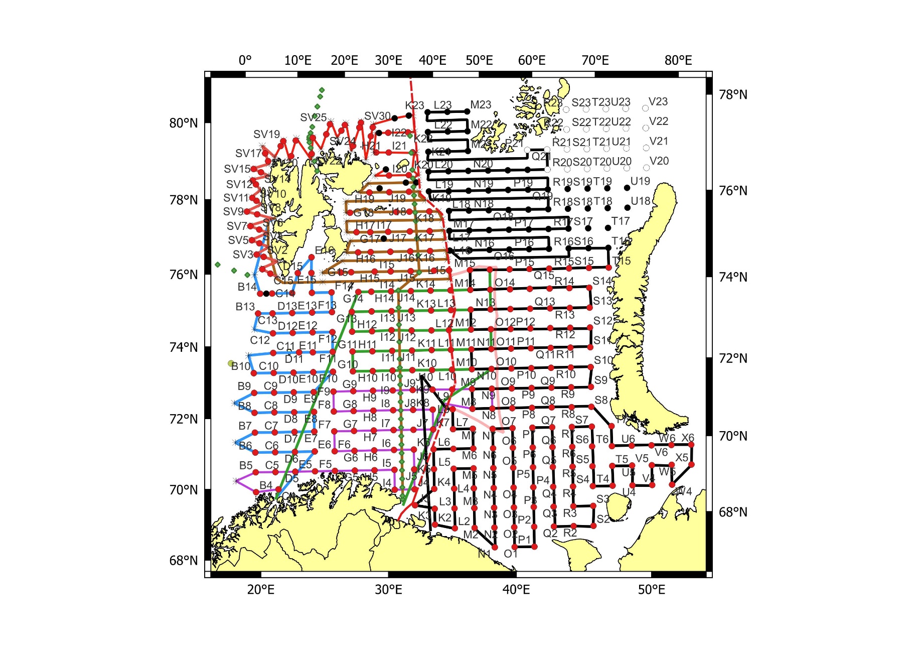
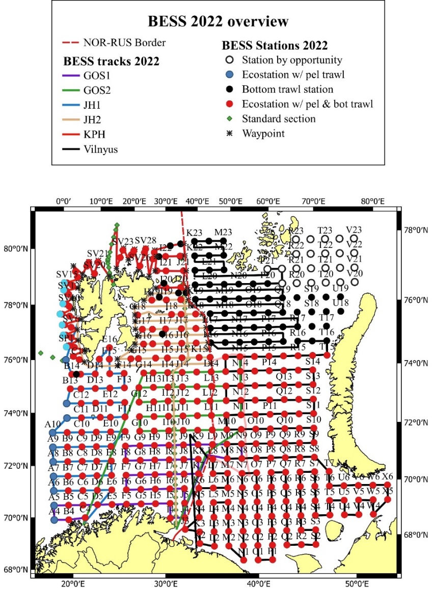
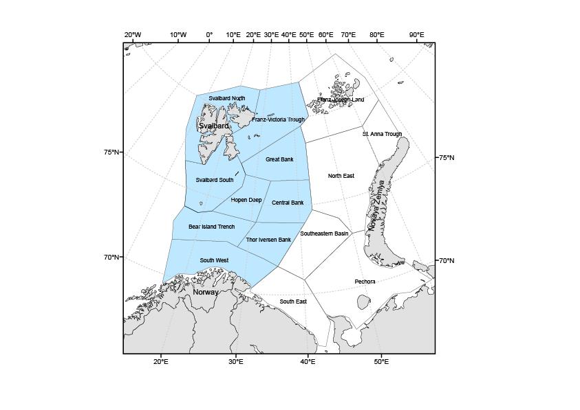
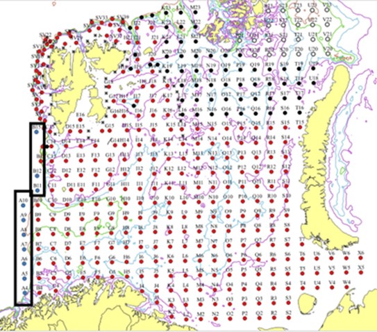
The combined Norwegian and Russian coverage (Figure 7.2, AII.2) is designed to start in south (ideally south-west) and progress northwards in a north-eastern direction. The survey covers the whole Barents Sea and the Svalbard area to max 500 m depth in the western and northern parts, except from some uncovered areas in the far north-east and south-east.
The vessel track lines proceed through the sampling stations, except in the area around Svalbard, where the tracks follow a zig-zag design and in the capelin area east of Svalbard where the tracks are denser.
Both the Norwegian and Russian part of the survey are vital to obtain a reasonable monitoring of the ecosystem components targeted by the survey. It is also important that these two parts progresses in a synoptic manner so that the time lag between stations and transects on each side of the NOR-RUS border is minimised. Synopsis in the Norwegian capelin area is also considered as the end of the Svalbard coverage must coincide with the end of the more southern coverage of the capelin area. Perfect synoptic coverage is rarely obtained since the design involves 4 vessels with change of crew and personnel at mid coverage on two of them, i.e. 6 vessel coverages that needs to be combined. There are also year-to-year deviations in the coverage due to external factors such as; weather, technical problems, insufficient funding etc.
Figure 7.2. AII.2. Typical geographical coverage of BESS (planned for 2022) showing geographical extent, station grid, and track lines.
7.1.3 - Stations and transects
Sampling at regular stations (i.e. ecosystem stations) covers almost all components monitored by the survey. The concept of an ecosystem station is vital for the survey. An ecosystem station involves observations of several ecosystem components at the same place and time (simultaneous observations). This enable analysis of the relationship between several components. A typical ecosystem station involves sampling with CTD, WPII, bottom trawl and pelagic trawl. In addition, some of the ecosystem stations also involves sampling with Multinet. See descriptions in Appendix IV for details about sampling.
In most of the Barents Sea, the ecosystem stations are arranged in a regular grid (35x35 nmi), based on an Albers equal-area projection. In the Svalbard area, the ecosystem stations are distributed within the two depth categories 100-300 m and 300-500 m along every other track of a zig-zag design. The tracks and location of these stations are design according to two geographic strata, one west and the other north of Svalbard, i.e. a pre-stratified design based on geography and depth.
Other stations are also covered by the survey, involving special bottom trawl stations for Greenland halibut, pelagic trawling on acoustic registrations, some microplastics stations between ecosystem stations, and stations taken as part of standard oceanographic sections.
The vessel tracks lines are optimised to serve as acoustic transects. They proceed through the sampling stations and are designed to stretch as far as possible in the east-west direction to facilitate acoustic estimation. Exceptions are the area around Svalbard, where the tracks follow a zig-zag design in two predefined strata, and in the capelin area east of Svalbard where additional acoustic transects are added between the lines defined by the sampling stations in a predefined geographic stratum. Three standard oceanographic sections (Vardø-Nord expanded, Sørkapp vest, and Hinlopen) are sampled as part of BESS. They serve as transects where the track lines proceed through several standard oceanographic stations to provide data for these.
7.1.4 - Ecosystem components covered by BESS
Here is a brief description of the ecosystem components covered by BESS. Detailed descriptions of these and the sampling methods involved are given in Appendix IV.
Pollution in biota and sediments: organic, non-organic pollutants, metals and other in fish, invertebrates, and sediment
Plankton community: species and biomass (transect), biomass and distribution of phyto, meso and macrozooplankton
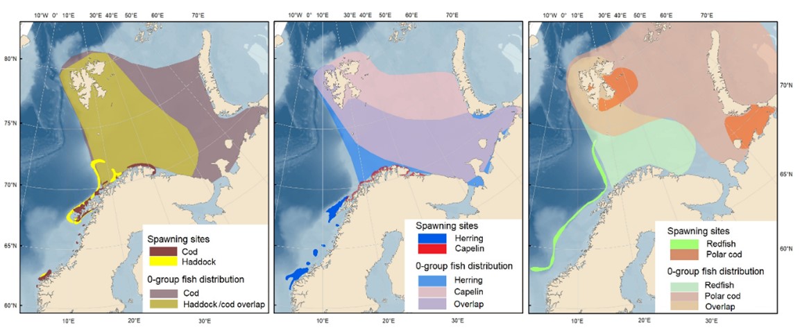
Fish recruitment (age 0): abundance, biomass, length and distribution of capelin, herring, cod, haddock, polar cod, saithe, Greenland halibut, beaked redfish, long rough dab
Pelagic fish stocks: capelin, young herring, blue whiting, and polar cod (abundance, biomass, length and age composition, condition, diet (capelin and polar cod), and distribution)
Demersal fish stocks: cod, haddock, saithe, redfish (2 species), wolffish (3 species) and Greenland halibut (abundance, biomass, length and age composition, condition, diet (cod), and distribution)
Fish community of non-commercial species: abundance, biomass, length and distribution
Commercially important invertebrates: northern shrimps, snow and king crabs (abundance, biomass, length, distribution)
Benthos: number of species, biomass and numbers. Length measures of particular vulnerable species.
Marine mammals: number of species observations along the cruise track
Sea birds: number of species observations along the cruise track
7.2 - BESS – deliverables and value
BESS represents a national treasure for marine science and advice in Norway, and the revenue from of BESS includes of both short-term and long-term values. Short-term values are in the form of assignments to BESS, to the institute (The Purpose- and Mission letter), requests from the Fisheries Agency, Environmental Agency, Petroleum directorate and others, and ongoing projects. Long-term values are in the form of data bases, increased expertise, ecosystem/species/interaction knowledge building, methodology development, or investment in the future project.
BESS has extensive interaction with many disciplines within IMR due to the broad and interdisciplinary focus of the survey. BESS also contributes with training of new cruise leaders and research technicians. The international collaboration during BESS is important for EU projects and other international project. The BESS has a unique collaboration with VNIRO (Russia) spanning from scientist and technician exchange to planning of BESS, time series calculation and reporting of results.
7.2.1 - Economical value
The BESS is a platform serving the entire IMR with necessary data collection. In the short term it saves money as a lot of activities is concentrated to one platform, which otherwise had to be conducted as single cruises. It also represents short-term values in the form of assignments to BESS, to the institute (The Purpose- and Mission letter), and other ongoing projects. In the long term, several projects belonging to different IMR’s Research and Advisory Programmes (the Barents Sea, the Norwegian Sea, the North Sea, Norwegian Coast, Marine processes, and Safe and Healthy Seafood) are dependent on BESS data or collection of own samples during BESS.
The BESS budget is, on a yearly basis, 4-6 times lower than the total budget for IMR projects it serves, and which depend on data from the survey (Figure 7.3 AII.3). This clearly demonstrates an important (and for some projects essential) role of the BESS as stable and secure investment into ongoing and future projects and thus IMR funding.
Figure 7.3 AII.3. The economic value of IMR projects relying on BESS as their data input source. The red line represents the IMR budget required every year to run BESS. On average BESS represents a yearly economic revenue of 4.5 times the cost for IMR.
7.2.2 - Data and time series
BESS collects data for hundreds of time series: stock assessment (biomass and abundance per age, condition, etc.), fish recruitment at age 0 (abundance for 11 species and biomass for 6), mesozoo- and macrozooplankton biomass on average and in space, non-commercial fish species and benthos species abundances and biomass on average and in space, other biological (biodiversity, fish diet, overlap, feeding conditions, etc.), and physical time series (temperature and salinity (surface, water column, at the bottom) on average and in space etc.). It is also a valuable source for simultaneous (in time and space) data for ecological studies.
7.2.3 - Advice
Output from BESS is used for several assessment purposes based on time series and spatial data resulting in advice to national ministries ((NFD, KLD, etc.) and international advisory and management organisations (Norwegian-Russian Environmental Commission, Arctic Council, OSPAR, etc.).
It provides over hundreds of time series used in 1) stock assessment of commercial fish and crustaceans and used by ICES working groups (AFWG, WGWIDE, …), 2) assessment of ecosystem status used by ICES working groups (WHOL…, WGIBAR, WGICA), and vulnerability (WGDEC) and, 3) provide valuable insight into annual and long-term variations in the ecosystem used by The Norwegian Management Plan, Arctic Council (PAME, AMAP, CBMP) and OSPAR. This is essential for assessing climate impacts on the various commercially and ecologically important stocks (IPCC 2022).
Data, time series and knowledge from the BESS have been used in national and international reports providing advice and/or knowledge for sustainable harvesting of living marine resources, environmental status and change, protection of marine areas and resources, and several others.
Thus, BESS clearly fulfils the IMR, national and international goals of developing towards ecosystem-based advice and management.
7.2.4 - New knowledge
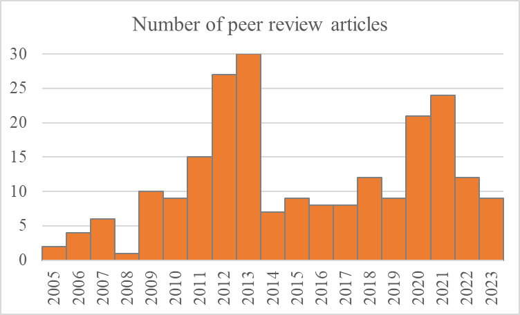
The BESS accumulated a new knowledge (documented by hundreds of papers) represents a valuable knowledge base for national and international marine sciences. The BESS data and time series are used in more than 200 per reviews articles, including several high ranged journals. On average 11 peer review articles published annually between 2005 and 2023 (Figure 7.4. AII.4).
Figure 7.4. AII.4. The number of peer review articles based on BESS data for period 2005 and 2023.
7.2.5 - IMR internal work culture
BESS contributes to the development of expertise of researchers and technicians at IMR within ecosystem-based monitoring, technology, survey methodology and taxonomy (hundreds of plankton, fish, and thousands of benthos species). During the surveys, multidisciplinary team work together with the sampling contributing to valuable knowledge transfer between different disciplines. This paves the way for further inter-disciplinary work at IMR in the long run.
7.3 - Development and innovation
BESS is a platform for developing new focus areas and new methodology for IMR. The efforts to make the survey as cost-effective as possible has been ongoing since the start of the survey in 2004. This has led to new ways of organising ecosystem monitoring by surveys, coordinating different equipment, effective onboard sampling and use of new technology. Some examples of new and planned development are given below.
7.3.1 - Snow crab
Snow crab monitoring is being changed to be carried out as part of the ecosystem tour and using AUV and image analysis. There will be increased use of data from fishing vessels. FG Benthic resources and processes is asked to develop a project description for an internal method project based on AUV and fishery-dependent data etc. which will be the basis for population assessment and advice on snow crab from and including 2024. Deadline 15 March.
7.3.2 - New gear for pelagic fish
The experience showing that the standard pelagic trawl Harstad trawl varied in opening with depths, while (Aakrahamn-trawl) used by Norwegian vessels to identify acoustically recorded fish such as herring, mackerel had low and variable catching efficiency. Therefore, a new pelagic survey trawl (VITO trawl) was designed by IMR in 2018 based on a commercial trawl targeting species such as herring, mackerel, capelin and saithe, and improving 0-group fish catch and time use.
During the BESS measurements of trawl geometry were performed and showed that the trawl had a vertical opening of approximately 35 m and a wingspread of approximately 28 m. Catch comparison between the Harstad-trawl (standard pelagic trawl) and the new pelagic trawl showed that the VITO-trawl has a potential both as a pelagic trawl to verify acoustically recorded fish and a trawl to be used for targeting 0-group fish. IMR planned to carry out comparisons between the Harstad-trawl and the VITO-trawl during BESS, but not performed due to cut founding.
7.3.3 - Benthos
New DNA methods are developing and may help identifying species from samples. One way to kick-start such a development would be to gene-code the species in the Barents Sea and to develop tools (sensors) that can be brought to sea and used in species identification.
7.3.4 - Seafood quality (Parasites)
Arctic marine ecosystems preserve a vast biodiversity. So far, parasites have been given little consideration in marine biodiversity although helminth parasites even exceed the biodiversity of their vertebrate hosts. Furthermore, parasites presence/abundance is indirectly affected by biotic and abiotic drivers, and marine host-parasite interactions constitute a relationship which can be dramatically impacted by global changes. Marine parasites can be used as biological indicators for the ecosystem they inhabit. Their presence/absence and abundance can be a valuable tool to monitor the effect of anthropogenic stressors on marine biodiversity. In particular, heteroxenous parasites with complex life cycle parasites (i.e., parasites that require multiple host species linked by a trophic-web to complete their life cycles), are dramatically subject to alterations of the marine ecosystems. Stressors affecting population dynamic of each single host could then affect parasite transmission success and be reflected as changes of parasite abundance and genetic variability. In addition, some marine parasites species particularly abundant in arctic and subarctic ecosystems may heavily impact seafood safety and quality of fish species with a high commercial value.
8 - Appendix III: Peer-Reviewed papers based on deliverables from BESS in the period 2005-2023
8.1 - References
8.1.1.1 -
2005
Jørgensen, LL. 2005. Impact scenario for an introduced decapod on Arctic epibenthic communities. Biological Invasions, 7(6), 949-957.
8.1.1.2 - 2006
Dingsør, GE. 2006. Influence of spawning stock size and environment on abundance of juveniles in commercially important fish stocks in the Barents Sea. Dr. Scient. dissertation, University of Bergen, 2006. http://hdl.handle.net/1956/1515
Fauchald, P., M. Mauritzen and H. Gjøsæter 2006. Density-dependent migratory waves in the marine pelagic ecosystem. Ecology, 87: 2915-2924.
Pedersen OP, Nilssen EM, Jørgensen LL, Slagstad D 2006. Advection of the Red King Crab larvae on the coast of North Norway – a Lagrangian model study. Fisheries Research 79:325-336
Slotte, A., Mikkelsen, N., and Gjøsæter, H. 2006. Egg cannibalism in Barents Sea capelin in relation to a narrow spawning distribution. Journal of Fish Biology 68:1-16.
8.1.1.3 - 2007
Ciannelli, L., G.E. Dingsør, B. Bogstad, G. Ottersen, K.-S. Chan, H. Gjøsæter, J.E. Stiansen and N.C. Stenseth. 2007. Spatial anatomy of species survival rates: effects of predation and climate-driven environmental variability. Ecology, 88 (3): 635-646.
Dingsør, G. E., Ciannelli, L., Chan, K.-S., Ottersen, G., Stenseth, N. C. 2007. Density dependence and density independence during the early life stages of four large marine fish stocks. Ecology 88 (3): 625-634.
Hjermann, D. Ø., A. Melsom, G. E. Dingsør, J. M. Durant, A. M. Eikeset, L. P. Røed, G. Ottersen, G. Storvik, and N. C. Stenseth. 2007. Fish and oil in the Lofoten-Barents Sea system: synoptic review of the effect of oil spills on fish populations. Marine Ecology-Progress Series 339:283-299.
Hjermann, D. Ø., Bogstad, B., Eikeset, A. M., Ottersen, G., Gjøsæter, H., and Stenseth, N. C. 2007. Food web dynamics affect Northeast Arctic cod recruitment. Proceedings of the Royal Society, Series B 274:661-669.
Jørgensen, Lis Lindal, and Raul Primicerio 2007. Impact scenario for the invasive red king crab Paralithodes camtschaticus (Tilesius, 1815) (Reptantia, Lithodidae) on Norwegian, native, epibenthic prey. Hydrobiologia 590.1: 47-54.
Svendsen, E., Skogen, M., Budgell, P., Huse, G., Ådlandsvik, B., Vikebø, F., Stiansen, J.E., Asplin, L., Sundby, S. 2007. An Ecosystem Modelling Approach to Predicting Cod Recruitment. Deep-Sea Research, part II, 54: 2810-2821.
8.1.1.4 - 2008
Ciannelli, L., P. Fauchald, KS. Chan, VN. Agostini, and GE. Dingsør. 2008. Spatial fisheries ecology: Recent progress and future prospects. Journal of Marine Systems 71(3-4): 223-236.
8.1.1.5 - 2009
Aschan, M. and Ingvaldsen, R., 2009. Recruitment of shrimp (Pandalus borealis) in the Barents Sea related to spawning stock and environment. Deep-Sea Research II 56 (2009), 2012-2022.
Dalpadado P., Bogstad B., Eriksen E and Rey L. 2009. Distribution and diet of 0-group cod (Gadus morhua) and haddock (Melanogrammus aeglefinus) in the Barents Sea in relation to food availability and temperature. Polar biol 32(11):1583-1596
Eriksen E., Prozorkevich D., Dingsør G., 2009. An evaluation of 0-group abundance indices of Barents Sea fish stocks, The Open Fish Science Journal, Volume 2, pp. 6-14.
Gjøsæter, H., B. Bogstad and S. Tjelmeland 2009. Ecosystem effects of the three capelin stock collapses in the Barents Sea. Marine Biology Research, 5: 40 - 53.
Haug, T., I. Røttingen, H. Gjøsæter, O.A. Misund, T. Fenchel and F. Uiblein 2009. Fifty years of Norwegian-Russian collaboration in marine research. Marine Biology Research, 5: 1 - 3.
Hjermann, D. Ø., B. Bogstad, G. E. Dingsør, H. Gjøsæter, G. Ottersen, A. M. Eikeset, and N. Chr. Stenseth. 2010. Trophic interactions affecting a key ecosystem component: a multi-stage analysis of the recruitment of the Barents Sea capelin. Canadian Journal of Fisheries and Aquatic Sciences 67(9): 1363–1375.
Lindstrøm, U., Smout, S., Howell, D., and Bogstad, B. 2009. Modelling multispecies interactions in the Barents Sea ecosystem with special emphasis on minke whales, cod, herring and capelin. Deep Sea Research Part II: Topological Studies in Oceanography 56: 2068-2079.
Link, J. S., Bogstad, B., Sparholt, H., and Lilly, G. R. 2009. Role of Cod in the Ecosystem. Fish and Fisheries 10(1):58-87.
Skern-Mauritzen, M., Skaug, H.J. and Øien, N. 2009. Line transects, environmental data and GIS: Cetacean distribution, habitat and prey selection along the Barents Sea shelf edge. NAMMCO Sci.Publ. 7:179-200.
Yaragina, N. A., Bogstad, B., and Kovalev, Yu. A. 2009. Reconstructing the time series of abundance of Northeast Arctic cod (Gadus morhua), taking cannibalism into account. In Haug, T., Røttingen, I.,
Gjøsæter, H., and Misund, O. A. (Guest Editors). 2009. Fifty Years of Norwegian-Russian Collaboration in Marine Research. Thematic issue No. 2, Marine Biology Research 5(1):75-85.
Agnalt, A.L., Jørstad, K.E., Pavlov V., Olsen E. 2010. Recent Trends in Distribution and Abundance of the Snow Crab (Chionoecetes opilio) Population in the Barents Sea. . In: Kruse GH, Eckert GL,
Foy RJ, Lipcius RN, Sainte-Marie B, Stram DL, Woodby D (eds) Biology and Management of Exploited Crab Populations under Climate Change University of Alaska, Fairbanks, p 317-327
8.1.1.6 - 2010
Dolgov, A., Johannesen, E., Heino, M. and Olsen. E. 2010. Trophic ecology of blue whiting in the Barents Sea. ICES Journal of Marine Science 67 : 483-493.
Hjermann, D. Ø., Bogstad, B., Dingsør, G. E., Gjøsæter, H., Ottersen, G., Eikeset, A. M., and Stenseth, N. C. 2010. Trophic interactions affecting a key ecosystem component: a multi-stage analysis of the recruitment of the Barents Sea capelin. Canadian Journal of Fisheries and Aquatic Science 67:1363-1375.
Howell, D., and Bogstad, B. 2010. A combined Gadget/FLR model for management strategy evaluations of the Barents Sea fisheries. ICES Journal of Marine Science 67:1998-2004.
Olsen, E., Aanes, S., Mehl, S., Holst, J.C., Aglen, A., and Gjøsæter, H., 2010. Cod, haddock, saithe, herring, and capelin in the Barents Sea and adjacent waters: a review of the biological value of the area. ICES Journal of Marine Science 67(1): 87-101. doi:10.1093/icesjms/fsp229
Reiss H, Greenstreet S, Robinson L, Ehrich S, Jørgensen LL, Piet GJ, Wolff WJ (2010). Unsuitability of TAC management within an ecosystem approach to fisheries: An ecological perspective. Journal of Sea Research 63:85-92
Smedsrud, L. H., R. Ingvaldsen, J.E.Ø. Nilsen, and Ø Skagseth., 2010. Heat in the Barents Sea: Transport, storage, and surface fluxes. Ocean Science, 6, 219-234.
Svetocheva O.N. and Eriksen E. 2010. Otholits of some demersal Barents Sea fishes (Lycodes and Cottidae). MMBI Press, Murmansk.
Westgård T., Johansen G.O., Kvamme C., Ådlandsvik B., and Stiansen J.E. 2010. A framework for storing, retrieving and analysing marine ecosystem data of different origin with variable scale and distribution in time and space. Pp. 417-432 in Nishida, T., and Caton, A.E. (Editors), GIS/Spatial Analyses in Fishery and Aquatic Sciences (Volume 4). International Fishery GIS Society, Saitama, Japan. 579 pp. (ISBN: 4-9902377-2-2).
8.1.1.7 - 2011
Anisimova NA, Jørgensen LL, Lubin P., Manushin I. (2011). Benthos. In: T. Jakobsen, V. Ozhigin (Edt.) The Barents Sea Ecosystem: Russian-Norwegian Cooperation in research and management, Chapter 4.1.2.
Eriksen E. and Dalpadado P. 2011. Long-term changes in Krill biomass and distribution in the Barents Sea: are the changes mainly related to capelin stock size and temperature conditions? Polar Biol 34(9):1399-1409, https://doi.org/10.1007/s00300-013-1357-x
Eriksen E., Bogstad B., Nakken O. 2011. Ecological significance of 0-group fish in the Barents Sea ecosystem. Polar Biol 34:647–657. https://doi.org/10.1007/s00300-010-0920-y
Eriksen, E. and Prozorkevich, D. 2011. 0-group survey. In: Jakobsen T and Ozhigin V (ed) The Barents Sea ecosystem, resources, management. Half a century of Russian-Norwegian cooperation. Tapir Academic Press, Trondheim, pp 557-569.
The Barents Sea - ecosystem, resources, management. Half a century of Russian - Norwegian cooperation. By Jakobsen, Tore; Ozhigin, Vladimir K. (Book, 2011)
Johansen, G.O, Johannesen, E., Michalsen, K. Aglen, A. and Fotland, Å. 2011. Seasonal variation in geographic distribution of NEA cod - survey coverage in a warmer Barents Sea, Marine Biology Research, 9: 908-919
Jørgensen LL, Nilssen E 2011. The alien marine crustacean of Norwegian coast; invasion history and impact scenario of the red king crab Paralithodes camtschaticus. In: B.S. Galil et al. (eds.), In the Wrong Place - Alien Marine Crustaceans: Distribution, 521 Biology and Impacts, Invading Nature - Springer Series in Invasion Ecology 6, DOI 10.1007/978-94-007-0591-3_18
Jørgensen LL, Renaud P, Cochrane S. (2011). Improving benthic monitoring by combining trawl and grab surveys. Marine Pollution Bulletin 62 1183-1190.
Kristiansen, T., Drinkwater, K. F., Lough, R. G. & Sundby, S. Recruitment Variability in North Atlantic Cod and Match-Mismatch Dynamics. 2011. Plos One 6, e17456
Michalsen K, Dalpadado P, Eriksen E, Gjøsæter H, Ingvaldsen R, Johannesen E, et al. 2011. The joint Norwegian–Russian ecosystem survey: overview and lessons learned Proceeding, of the 15th Norwegian–Russian Symposium, Longyearbyen, Norway, 6–9 September 2011, p 247 – 272.
Olsen, E., Michalsen, K., Ushakov, N.G., Zabavnikov, V.B. 2011. The ecosystem survey. In The Barents Sea. Ecosystem, resources, management. Half a century of Russian-Norwegian cooperation, pp. 604-608. Ed. by T. Jakobsen. and V.K. Ozhigin, V.K. Tapir Academic Press, Trondheim
Planque, B., Bellier, E., and Loots, C. 2011. Uncertainties in projecting spatial distributions of marine populations. ICES Journal of Marine Science, 68: 1045-1050.
Planque, B., Loots, C., Petitgas, P., Lindstrøm, U., and Vaz, S. 2011. Understanding what controls the spatial distribution of fish populations using a multi-model approach. Fisheries Oceanography, 20: 1-17.
Mette Skern-Mauritzen, Edda Johannesen, Arne Bjørge, Nils Øien.2011. Baleen whale distributions and prey associations in the Barents Sea. Marine Ecology Progress Series. Vol. 426: 289–301, 201. doi:10.3354/meps09027
Vikebø FB, Ådlandsvik B, Albretsen J, Sundby S, Stenevik EK, Huse G, Svendsen E, Kristiansen T, Eriksen E. 2011. Real-Time Ichthyoplankton Drift in Northeast Arctic Cod and Norwegian Spring-Spawning Herring. PLoS ONE 6(11): e27367. https://doi.org/10.1371/journal.pone.0027367
Årthun, M., Ingvaldsen, R.B., Smedsrud, L.H., Schrum C., 2011. Dense water formation and circulation in the Barents Sea. Deep-Sea Research I 58, 801-817.
8.1.1.8 - 2012
Baulier, L., Heino, M., and Gjøsæter, H. 2012. Temporal stability of the maturation schedule of capelin Mallotus villosus in the Barents Sea. Aquatic Living Resources, 25: 151-161.
Bluhm BA, J.M. Grebmeier, P. Archambault, M. Blicher, G. Guðmundsson, K. Iken, L. Lindal Jørgensen, V. Mokievsky 201). Benthos. In: Jeffries, M. O., J. A. Richter-Menge and J. E. Overland, Eds., 2012: Arctic Report Card 2012, http://www.arctic.noaa.gov/reportcard.
Condon R.H., Duarte C.M., Pitt K.A., Robinson K.L., Lucas C.H., Sutherland K.R., Mianzan H.W., Bogeberg W., Purcell J.R, Decker M.B., Uye S., Madin L.P., Brodeur R.D., Haddock S.H.D., Malej A., Parry G.D., Eriksen E., Quiñones J., Acha M., Harvey M., Arthur J.A., and Graham W.M. 2012. Recurrent jellyfish blooms are a consequence of global oscillations. Proceedings of the National Academy of Sciences 110(3): 1000-1005. https://doi.org/10.1073/pnas.1210920110
Dalpadado, P., Ingvaldsen, R. B., Stige, L. C., Bogstad, B., Knutsen, T., Ottersen, G., and Ellertsen, B. 2012. Climate effects on the Barents Sea ecosystem dynamics. ICES Journal of Marine Science 69 (7):1303-1316.
Eriksen E, Ingvaldsen R, Stiansen JE, Johansen GO. 2012. Thermal habitat for 0-group fishes in the Barents Sea; how climate variability impacts their density, length and geographical distribution. ICES Journal of Marine Science, 69(5): 870–879. https://doi.org/10.1093/icesjms/fsr210
Eriksen E, Prozorkevich D, Trofimov A, Howell D 2012. Biomass of Scyphozoan Jellyfish, and Its Spatial Association with 0-Group Fish in the Barents Sea. PLoS ONE 7(3): e33050. https://doi.org/10.1371/journal.pone.0033050
Eriksen E., Prokhorova T., and Johannesen E. 2012. Long term changes in abundance and spatial distribution of pelagic Agonidae, Ammodytidae, Liparidae, Cottidae, Myctophidae and Stichaeidae in the Barents Sea. In: M. Ali (ed.) Diversity of Ecosystems, ISBN: 978-953-51-0572-5, InTech, Croatia, pp 107-126.
Fevolden, S-E; Westgaard, J-I; Pedersen, T; Præbel, K 2012. Settling-depth vs. genotype and size vs. genotype correlations at the Pan I locus in 0-group Atlantic cod Gadus morhua. Marine Ecology Prog. Ser. VOL 468: 267-278. doi: 10.3354/meps09990
Friedland, K, Stock, C, Drinkwater, K, Link, JS. Leaf, RT, Shank, BV. Rose, JM. Pilskaln, CH. Fogarty, MJ. 2012. Pathways between Primary Production and Fisheries Yields of Large Marine Ecosystems. PloSOne, January 20, 2012 ttps://doi.org/10.1371/journal.pone.0028945
Fu, C; Gaichas, S; Link, JS.; Bundy, A; Boldt, JL.; Cook, AM.; Gamble, R; Utne, KR; Liu, H; Friedland, K. 2012. Relative importance of fisheries, trophodynamic and environmental drivers in a series of marine ecosystems. Marine Ecology Progress Series, Vol. 459 (July 12 2012), pp. 169-184. https://www.jstor.org/stable/24876324
Gjøsæter, H., S. Tjelmeland and B. Bogstad 2012. Ecosystem-Based Management of Fish Species in the Barents Sea. In Global Progress in Ecosystem-Based Fisheries Management., pp. 333-352. Ed. by G. H. Kruse, HI. Browman, KL. Cochrane, D. Evans, GS. Jamieson, PA. Livingston, D. Woodby and CI. Zhang. Alaska Sea Grant, University of Alaska Fairbanks
Golikov AV, Sabirov RM, Lubin PA, Jørgensen LL 2012. Changes in distribution and range structure of Arctic cephalopods due to climatic changes of the last decades. Biodiversity1:1-8
Gwynn, J. P., Heldal, H. E., Gäfvert, T., Blinova, O., Eriksson, M., Sværen, I., Brungot, A. L., Strålberg, E., Møller, B., Rudjord, A. L., 2012. Radiological status of the marine environment in the Barents Sea. J. Environ. Radioact. 113, 155-62.
Johannesen E, Høines ÅS, Dolgov AV, Fossheim M 2012 Demersal Fish Assemblages and Spatial Diversity Patterns in the Arctic-Atlantic Transition Zone in the Barents Sea. PLoS ONE 7(4): e34924. doi:10.1371/journal.pone.0034924
Johannesen, E., Ingvaldsen, R., Dalpadado. P., Skern-Mauritzen, M., Stiansen, J.E., Eriksen, E., Gjøsæter, H., Bogstad, B. and Knutsen, T. 2012. Barents Sea ecosystem state: climate fluctuations, human impact and trophic interactions. ICES J. Mar. Sci. 69 (5): 880-889. https://doi.org/10.1093/icesjms/fss046
Johannesen, E., Lindstrøm, U., Michalsen, K., Skern-Mauritzen, M., Fauchald, P., Bogstad, B., and Dolgov, A. V. 2012. Feeding in a heterogeneous environment: spatial dynamics in summer foraging Barents Sea cod. Marine Ecology Progress Series 458:181-197.
Lind, S. and Ingvaldsen, R.B., 2012. Variability and impacts of Atlantic Water entering the Barents Sea from the north. Deep-Sea Research, I 62 (2012), 70-88. doi:10.1016/j.dsr.2011.12.007.
Meager, Justin J.; Skjæraasen, Jon Egil; Karlsen, Ørjan; Løkkeborg, Svein; Mayer, Ian; Michalsen, Kathrine; Nilsen, Trygve; Fernö, Anders 2012. Environmental regulation of individual depth on a cod spawning ground. Journal article; Peer reviewed, 2012-12-13
Michalsen, K., Dalpadado, P., Eriksen, E., Gjøsæter, H., Ingvaldsen, R.B., Johannesen, E., Jørgensen, L.L., Knutsen, T., Prozorkevich. D., andd Skern-Mauritzen, M.2012. Eight years of ecosystem surveys in the Barents Sea – Review and recommendations. Invited Review in Marine Biology Research.
Moksness, E., Link, JS. Drinkwater, K, Gaichas, S 2012. Bernard Megrey: pioneer of Comparative Marine Ecosystem analyses. Marine Ecology Progress Series Vol. 459 (July 12 2012), pp. 159-163. https://www.jstor.org/stable/24876322
Planque, B., Johannesen, E., Drevetnyak, K. V., and Nedreaas, K. H. 2012. Historical variations in the year-class strength of beaked redfish (Sebastes mentella) in the Barents Sea. – ICES Journal of Marine Science, doi:10.1093/icesjms/fss014.
Pranovi, Fabio; Link, Jason S.; Fu, Caihong; Cook, Adam M.; Liu, Hui; Gaichas, Sarah; Friedland, Kevin; Utne, Kjell R.; Benoît, Hugues P. 2012. Trophic-level determinants of biomass accumulation in marine ecosystems. Marine Ecology Progress Series, Vol. 459 (July 12 2012), pp. 185-202. https://www.jstor.org/stable/24876325
Saher M, Kristensen DK, Hald M, Pavlova O, Jørgensen LL 2012. Changes in distribution of calcareous benthic foraminifera in the central Barents Sea between the periods 1965-1992 and 2005-2006. Global and Planetary Change 98-99:81-96
Tsubouchi, T, Bacon, S, Garabato, AC, Naveira;Aksenov, Y, Laxon, SW, Fahrbach, E, Beszczynska-Möller, A, Hansen, E, Lee, CM, Ingvaldsen, R 2012. The Arctic Ocean in summer: A quasi-synoptic inverse estimate of boundary fluxes and water mass transformation. Journal of Geophysical Research: Oceans. Volume 117, Issue C1 https://doi.org/10.1029/2011JC007174
8.1.1.9 - 2013
Aschan, M, Fossheim, M, Greenacre, M, Primicerio, R 2013. Change in Fish Community Structure in the Barents Sea. PloSOne 2013. https://doi.org/10.1371/journal.pone.0062748
Bogstad, B, Dingsør, GE, Ingvaldsen, RB, Gjøsæter, H 2013. Changes in the relationship between sea temperature and recruitment of cod, haddock and herring in the Barents Sea. Marine Biology Research, doi: 10.1080/17451000.2013.775451
Carscadden, J.E., H. Gjøsæter and H. Vilhjálmsson. 2013. A comparison of recent changes in distribution of capelin (Mallotus villosus) in the Barents Sea, around Iceland and in the Northwest Atlantic. Progress in Oceanography. 114: 64–83
Durant, JM, Hjermann, DØ, Falkenhaug, T, Gifford, DJ, Naustvoll, LJ, Sullivan, BK, Beaugrand, G, Stenseth, NC 2013. Extension of the match-mismatch hypothesis to predator-controlled systems. by (Journal article; Peer reviewed, 2013-01-31)
Eikeset, AM, Richter, A, Dunlop, Erin S, Dieckmann, U, Stenseth, NC 2013. Economic repercussions of fisheries-induced evolution. PNAS 110: 12259-12264. https://doi.org/10.1073/pnas.121259311
Erikstad, KE, Reiertsen, TK, Barrett, RT, Vikebø, F, Sandvik, H 2013. Seabird−fish interactions: the fall and rise of a common guillemot Uria aalge population. Marine Ecology Prog. Ser VOL 475: 267-276. doi: 10.3354/meps10084
Glover, KA, Kanda, Naoisha; Haug, Tore; Pastene, Luis A; Øien, Nils; Seliussen, Bjørghild Breistein; Sørvik, Anne Grete Eide; Skaug, Hans Julius 2013. Hybrids between common and Antarctic minke whales are fertile and can back-cross. BMC Geetics, VOL 14: 25(2013). https://doi.org/10.1186/1471-2156-14-25
Hauge, KH, Blanchard, A, Andersen, G, Boland, R, Grøsvik, B-E, Howell, D, Meier, S, Olsen, E, Vikebø, F 2013. Inadequate risk assessments – A study on worst-case scenarios related to petroleum exploitation in the Lofoten area. Marine Policy, VOL 44: 82-89. https://doi.org/10.1016/j.marpol.2013.07.008
Heldal, HE, Vikebø, F and Johansen, GO 2013. Dispersal of the radionuclide cesium-137 (137Cs) from point-sources in the Barents and Norwegian Seas and its potential contamination of the Arctic marine food chain: Coupling numerical ocean models with geographical fish distribution data. Environm. Poll. 180, 190-198.
Hop, H. and Gjøsæter, H 2013. Polar cod (Boreogadus saida) and capelin (Mallotus villosus) as key species in marine food webs of the Arctic and the Barents Sea. Marine Biology Research. 9(9): 878-894.
Howell, D., Filin, AA, Bogstad, B and Stiansen, JE 2013. Unquantifiable uncertainty in projecting stock response to climate change: Example from North East Arctic cod. Marine Biology Research, 9:9, 920-931, http://dx.doi.org/10.1080/17451000.2013.775452
Huserbråten, MBO; Moland, E, Knutsen, H, Olsen, EM, André, C,; Stenseth, NC. 2013. Conservation, Spillover and Gene Flow within a Network of Northern European Marine Protected Areas. PloSOne (2013) https://doi.org/10.1371/journal.pone.0073388
Ingvaldsen, RB, Gjøsæter, H 2013. Responses in spatial distribution of Barents Sea capelin to changes in stock size, ocean temperature and ice cover. Marine Biology Reserach VOL 9 - Thematic Issue No. 7 Climate Effects on the Barents Sea Marine Living Resources. https://doi.org/10.1080/17451000.2013.775450
Josefson AB, Mokievsky V, Bergmann M, Blicher ME, Bluhm B, Cochrane S, Denisenko NV, Hasemann C, Jørgensen LL, Klages M, Schewe I, Sejr MK, Soltwedel T, Wesławski JM, Włodarska-
Kowalczuk M 2013. Marine invertebrates, chapter 8. In: Arctic Biodiversity Assessment, Status and Trends in Arctic Biodiversity. http://www.arcticbiodiversity.is/index.php/the-report/chapters/marine-invertebrates
Lien, VS, Trofimov, AG 2013. Formation of Barents Sea Branch Water in the north-eastern Barents Sea. Polar Research 32. https://doi.org/10.3402/polar.v32i0.18905
Lien, VS, Vikebø, FB, Skagseth, Ø 2013. One mechanism contributing to co-variability of the Atlantic inflow branches to the Arctic. Nat Commun 4, 1488 (2013). https://doi.org/10.1038/ncomms2505
Lydersen, C, Øien, N, Mikkelsen, B, Bober, S, Fisher, D, Kovacs, KM.2013. A white humpback whale (Megaptera novaeangliae) in the Atlantic Ocean, Svalbard, Norway, August 2012. Polar Research Vol 32 (2013). https://doi.org/10.3402/polar.v32i0.19739
Macaulay, GJ, Peña, H, Fässler, SMM, Pedersen, G, Ona, E 2013. Accuracy of the Kirchhoff-Approximation and Kirchhoff-Ray-Mode Fish Swimbladder Acoustic Scattering Models. PlosOne (2013) https://doi.org/10.1371/journal.pone.0064055
Michalsen K, Dalpadado P, Eriksen E, Gjøsæter H, Ingvaldsen RB, Johannesen E, Jørgensen LL, Knutsen T, Prozorkevich D, and Skern-Mauritzen, M 2013. Marine living resources of the Barents Sea – Ecosystem understanding and monitoring in a climate change perspective, Marine Biology Research, 9 (9) 932-947. https://doi.org/10.1080/17451000.2013.775459
Misund, OA, Olsen, E 2013 Lofoten–Vesterålen: for cod and cod fisheries, but not for oil? ICES Journal of Marine Science VOL 70: 722-725.
Ozerov, M, Vasemägi, A, Wennevik, V, Diaz-Fernandez, R, Kent, M, Gilbey, J, Prusov, S, Niemelä, E, Vähä, J-P, 2013. Finding Markers That Make a Difference: DNA Pooling and SNP-Arrays Identify Population Informative Markers for Genetic Stock Identification. PLoS One (2013) doi: 10.1371/journal.pone.0082434
Smedsrud, LH, Esau, I, Ingvaldsen, RB, Eldevik, T, Haugan, PM, Li, C, Lien, VS, Olsen, A, Omar, AM, Otterå, OH, Risebrobakken, B, Sandø, AB, Semenov, VA, Sorokina, S 2013. A.The role of the Barents Sea in the Arctic climate system. Reviews of Geophysics, VOL 51, Issue 3 p. 415-449 https://doi.org/10.1002/rog.20017
Svetocheva, ON, and Eriksen, E 2013. Morphological Ch 2013. aracteristics of the Demersal Fish Otoliths. Herald of the Kola Science Centre of the Russian Academy of Sciences, 4: 91-104, http://www.kolasc.net.ru/russian/news/vestnik/vestnik-4-2013.pdf (In Russian).
Tjensvoll, I, Kutti, T, Fosså, JH, Bannister, R 2013. Rapid respiratory responses of the deep-water sponge Geodia barretti exposed to suspended sediments. Aquatic Biology VOL. 19: 65-73. doi: 10.3354/ab00522
van der Meeren, T, Dahle, G, Paulsen, OI 2013. A rare observation of Atlantic halibut larvae (Hippoglossus hippoglossus) in Skjerstadfjorden, North Norway. Marine Biodiversity Records , Volume 6 , 2013, https://doi.org/10.1017/S1755267213000511
Vollset, KW, Catalán, IA, Fiksen, Ø, Folkvord, A 2013. Effect of food deprivation on distribution of larval and early juvenile cod in experimental vertical temperature and light gradients. By Marine Ecology Prog. Ser. 475: 191-201. htpps://doi: 10.3354/meps10129
Voronkov, A, Hop, H, Gulliksen, B 2013. Diversity of hard-bottom fauna relative to environmental gradients in Kongsfjorden, Svalbard. Polar Research 2013, 32, 11208, http://dx.doi.org/10.3402/polar.v32i0.11208
Ware, C, Berge, J, Sundet, JH, Kirkpatrick, JB, Coutts, ADM, Jelmert, A, Olsen, SM, Floerl, O, Wisz, MS, Alsos, IG. 2013. Climate change, non-indigenous species and shipping: assessing the risk of species introduction to a high-Arctic archipelago.Biodiversity Research. https://DOI: 10.1111/ddi.12117
Øigård, TA, Lindstrøm, U, Haug, T, Nilssen, KT, Smout, S 2013. Functional relationship between harp seal body condition and available prey in the Barents Sea. Marine Ecology Prog. SEr. 484: 287-301. https://doi: 10.3354/meps10272
8.1.1.10 - 2014
Eriksen, E., Durif C.M.F., and Prozorkevich, D. 2014. Lumpfish (Cyclopterus lumpus) in the Barents Sea: development of biomass and abundance indices, and spatial distribution. ICES J. Mar. Sci. 71(9): 2398–2402. https://doi.org/10.1093/icesjms/fsu059
Fall, J and Skern-Mauritzen, M (2014) White-beaked dolphin distribution and association with prey in the Barents Sea, Marine Biology Research, 10:10, 957-971, DOI: 10.1080/17451000.2013.872796
Landa, C.S., Ottersen, G., Sundby, S., Dingsør, G.E. and Stiansen, J.E. 2014. Recruitment, distribution boundary and habitat temperature of an arcto-boreal gadoid in a climatically changing environment – a case study on Northeast Arctic haddock (Melanogrammus aeglefinus). Fisheries Oceanography 23(6): 506-520. DOI: 10.1111/fog.12085
Planque, B., R. Primicerio, K. Michalsen, M. Aschan, G. Certain, P. Dalpadado, H. Gjøsæter, C. Hansen, E. Johannesen, L. L. Jørgensen, I. Kolsum, S. Kortsch, L. M. Leclerc, L. Omli, and M. Skern-Mauritzen. (2014). Who eats whom in the Barents Sea: a foodweb topology from plankton to whales. Ecology 95 (5). P 1430.
Kjesbu, O. S., Bogstad, B., Devine, J. A., Gjøsæter, H., Howell, D., Ingvaldsen, R., Nash, R. D. M, and Skjæraasen, J. E. 2014. Synergies between climate and management for Atlantic cod fisheries at high latitudes. Proceedings National Academy of Science 111 (9): 3478-3483.
Underwood, M.J., Rosen, S., Engås, A., Eriksen, E. (2014) Deep Vision: An In-Trawl Stereo Camera Makes a Step Forward in Monitoring the Pelagic Community. PLoS ONE 9(11): e112304. https://doi.org/10.1371/journal.pone.0112304
Wiedmann MA, Aschan M, Certain G, Dolgov, AV, Greenacre M, Johannesen E., Planque B and Primicerio R. 2014. Functional diversity of the Barents Sea fish community. Marine Ecology progress series 495: 205–218.
8.1.1.11 - 2015
Certain, G., Jørgensen, L.L., Christel, I., Planque, B., Vinceny, B. (2015). Mapping the vulnerability of animal community to pressure in marine systems: Disentangling impact types and integrating their effect from the individual to the community level. ICES Journal of Marine Science. Doi:10.1093/icesjms/fsv003.
Eriksen, E. 2015. Do scyphozoan jellyfish limit the habitat of pelagic species in the Barents Sea during the late feeding period? ICES J Mar Sci ICES 73(2): 217-226. https://doi.org/10.1093/icesjms/fsv183
Eriksen, E., Ingvaldsen, R. B., Nedreaas, K. and Prozorkevich, D. 2015. The effect of recent warming on polar cod and beaked redfish juveniles in the Barents Sea. Regional Studies in Marine Science 2: 105–112.
Fossheim M, Primicerio R, Johannesen E, Ingvaldsen RB, Aschan M and Dolgov AV. 2015. Recent warming leads to a rapid borealization of fish communities in the Arctic. Nature Climate Change5: 673–677
Ingvaldsen RB, Bogstad B, Dolgov AV, Ellingsen KE, Gjøsæter H, Gradinger R, Johannesen E, Tveraa T, and Yoccoz NG. 2015. Modelled and observed cod distributions. Nature Climate Change 5: 788-789
Jørgensen L.L, Ljubin P, Skjoldal HR, Ingvaldsen RB, Anisimova N, Manushin I. (2015). Distribution of benthic megafauna in the Barents Sea: baseline for an ecosystem approach to management. ICES Journal of Marine Science; 72 (2): 595-613
Jørgensen LL, Philippe Archambault, Claire Armstrong, Andrey Dolgov, Evan Edinger, Grant Gilchrist, Jon Hildebrand, Dieter Piepenburg, Walker Smith, Cecilie Quillfeldt, Michael Vecchione, Jake Rice (2015c). Arctic Ocean. Chapter 36G in: A Regular Process for Global Reporting and Assessment of the State of the Marine Environment, including Socio-economic Aspects (Regular Process). World Ocean Assessment. Ocean & Law of the Sea. UN. http://www.un.org/depts/los/global_reporting/WOA_RegProcess.htm
Renaud P, Løkken TS, Jørgensen LL, Berge J, Johnson BJ (2015) Macroalgal detritus and food-web subsidies along an Arctic fjord depth-gradient. Frontiers doi: 10.3389/fmars.
Zimina, O. L., Lyubin, P. A., Jørgensen, L. L., Zakharov, D. V., Lyubina, O. S., (2015). Decapod Crustaceans of the Barents Sea and adjacent waters: species composition and peculiarities of distribution. Arthropoda Selecta 24(3): 417–428
8.1.1.12 - 2016
Bogstad, B., Yaragina, N. A., and Nash, R. D. M. 2016. The early life-history dynamics of Northeast Arctic cod: levels of natural mortality and abundance during the first three years of life. Canadian Journal of Fisheries and Aquatic Science 73(2): 246-256.
Degen R., Jørgensen L., Ljubin P., Ellingsen I., Pehlke H., Brey T 2016. Patterns and drivers of megabenthic secondary production on the Barents Sea shelf, Marine Ecology Progress Series, 546, pp. 1-16. doi: 10.3354/meps11662
Eriksen, E., Skjoldal, H.R., Dolgov, A.V., Dalpadado, D., Orlova, E.L., Prozorkevich, D.V. 2016. The Barents Sea euphausiids: methodological aspects of monitoring and estimation of abundance and biomass. ICES J. Mar. Sci. 73(6): 1533–1544. https://doi.org/10.1093/icesjms/fsw022
Johannesen E., Jørgensen L.L., Fossheim M., Primicerio R., Greenacre M., Ljubin P.A., Dolgov A.V., Ingvaldsen R.B., Anisimova N.A., Manushin, I.E. (2016) Consistent large-scale patterns in community structure of benthos and fish in the Barents Sea. Polar Biology DOI 10.1007/s00300-016-1946-6.
Jørgensen L.L, Planque B, Thangstad TH, Certain G (2016). Vulnerability of megabenthic species to trawling in the Barents Sea. ICES Journal of Marine Science. DOI: 10.1093/icesjms/fsv107.
Kvamsdal, S.F., Eide, A., Ekerhovd, N-A., Enberg, K., Gudmundsdottir, A., Hoel, A. H., Mills, K.E., Mueter, F.J., Ravn-Jonsen, L., Sandal, L.K., Stiansen, J.E. and Vestergaard, N. 2016. Harvest control rules in modern fisheries management. Elementa: Science of the Anthropocene, 4:000114, doi: 10.12952/journal.elementa.000114
Gjøsæter, H., Hallfredsson, E. H., Mikkelsen, N., Bogstad, B., and Pedersen, T. 2016. Predation on early life stages is decisive for year class strength in the Barents Sea capelin (Mallotus villosus) stock. ICES Journal of Marine Science 73(2):182-195.
Lacharité M., Jørgensen L.L., Metaxas A., Lien V.S., Skjoldal H.R. 2016. Delimiting oceanographic provinces to determine drivers of spatial mesoscale patterns in offshore shelf benthic megafauna: a case study in the Barents Sea. Progress in Oceanography 146: 187-198
8.1.1.13 - 2017
Boitsov, Stepan; Grøsvik, Bjørn Einar; Klungsøyr, Jarle. 2017. Decreased or stabilised levels of contaminants in Norwegian waters. Fram Forum 2017 ;Volum 2017. s. 52-55
Eriksen, E. 2017. Dynamics of the Barents Sea pelagic compartment: species distributions, interactions and response to climate variability. Doctoral thesis, University in Bergen, http://bora.uib.no/handle/1956/15487
Eriksen, E., Skjoldal, H.R. Gjøsæter, H. and Primicerio R. 2017. Spatial and temporal changes in the Barents Sea pelagic compartment during the recent warming. Progress in Oceanography 151: 206-226, http://dx.doi.org/10.1016/j.pocean.2016.12.009
Frainer, A., Primicerio, R., Kortsch, S., Aune, M., Dolgov, A. V., Fossheim, M., and Aschan, M. M. 2017. Climate-driven changes in functional biogeography of Arctic marine fish communities. Proceedings of the National Academy of Sciences: 201706080
Haug, T., Bogstad, B., Chierici, M., Gjøsæter, H., Hallfredsson, E. H., Høines, Å. S., Hoel AH., Ingvaldsen R.B., Jørgensen L.L., Knutsen T., Loeng H., Naustvoll L.J., Røttingen I., Sunnanå K., Loeng, H. (017. Future harvest of living resources in the Arctic Ocean north of the Nordic and Barents Seas: A review of possibilities and constraints. Fisheries Research, 188, 38-57.
Jørgensen (2017) Trawl and temperature pressure on Barents benthos. FEATURE ARTICLE – ICES, 11 July 2017
Jørgensen, LL., Archambault P., Blicher M., Denisenko N., Guðmundsson G., Iken K., Roy V., Sørensen J., Anisimova N., Behe C., Bluhm B.A., Denisenko S., Denisenko N., Metcalf V., Olafsdóttir S., Schiøtte T., Tendal O., Ravelo A.M., Kędra M., Piepenburg D. 2017. "Benthos" In: CAFF. State of the Arctic Marine Biodiversity Report. Conservation of Arctic Flora and Fauna, Akureyri Iceland.
Zakharov, D.V. and Jørgensen, L.L., 2017. New species of the gastropods in the Barents Sea and adjacent waters. Russian Journal of Biological Invasions, 8(3), pp.226-231.
8.1.1.14 - 2018
Bergstad, O.A., Johannesen, E., Høines, Høines, Åge, Ellingsen, Kari E., Lien, Vidar S., Byrkjedal, Ingvar, Yoccoz, Nigel G., Tveraa, Torkild, Wienerroither, Rupert, Langhelle, Gunnar, de Lange Wenneck, Thomas (2018) Demersal fish assemblages in the boreo-Arctic shelf waters around Svalbard during the warm period 2007–2014. Polar Biol 41, 125–142https://doi.org/10.1007/s00300-017-2176-2
Eriksen, E., Bogstad, B., Dolgov, A., Beck, I.M. 2018. Cod diet as an indicator of Ctenophora abundance dynamics in the Barents Sea. Mar Ecol Prog Ser 591:87-100. https://doi.org/10.3354/meps12199
Eriksen, E., Gjøsæter, H., Prozorkevich, D., Shamray, E. , Dolgov, A., Skern-Mauritzen, M., Stiansen, J.E., Kovalev, Yu., and Sunnanå, K., 2018. From single species surveys towards monitoring of the Barents Sea ecosystem, Progr. Oceanogr., Vol 166, 4-14. doi: 10.1016/j.pocean.2017.09.007.
Fall J, Ciannelli L, Skaret G, Johannesen E (2018) Seasonal dynamics of spatial distributions and overlap between Northeast Arctic cod (Gadus morhua) and capelin (Mallotus villosus) in the Barents Sea. PLOS ONE 13: e0205921. https://doi.org/10.1371/journal.pone.0205921
Grøsvik, B.E., Prokhorova, T., Eriksen, E., Krivosheya, P., Horneland, P.A., Prozorkevich, D. 2018. Assessment of marine litter in the Barents Sea, a part of the joint Norwegian-Russian ecosystem survey. Front. Mar. Sci., 06 March 2018. https://doi.org/10.3389/fmars.2018.00072
Gwynn, J. P., Heldal, H. E., Flo, J. K., Sværen, I., Gäfvert, T., Haanes, H., Føyn, L., Rudjord, A. L., 2018. Norwegian monitoring (1990–2015) of the marine environment around the sunken nuclear submarine Komsomolets. J. Environ. Radioact. 182, 52-62.
Levsen, A., Svanevik, C.S., Cipriani, P., Mattiucci, S., Gay, M., Hastie, L.C., Bušelić, I., Mladineo, I., Karl, H., Ostermeyer, U., Buchmann, K., Højgaard, D., González, A.F., Pascual, S., Pierce, G.J. 2018. A survey of zoonotic nematodes of commercial key fish species from major European fishing grounds – Introducing the FP7 PARASITE exposure assessment study. Fisheries Research 202, 4-21
Lind, S., Ingvaldsen, R. B., & Furevik, T. 2018. Arctic warming hotspot in the northern Barents Sea linked to declining sea-ice import. Nature Climate Change, 8(7), 634-639. https://doi.org/10.1038/s41558-018-0205-y
Pedersen T, Fuhrmann MM, Lindstrøm U, Nilssen EM, Ivarjord T, Ramasco V, Jørgensen LL, Sundet JH, Sivertsen K, Källgren E., Hjelset AM, Michaelsen C, Systad G, Norrbin F, Svenning A, Bjørge A, Steen H, Nilssen T 2018. Effects of the invasive red king crab on food web structure and ecosystem properties in an Atlantic fjord. Marine Ecology Progress Series, 596, 13-31.
Aarflot J, Aksnes D, Opdal A, Skjoldal HR, Fiksen Ø (2018). Caught in broad daylight: Topographic constraints of zooplankton depth distributions. Limnology and Oceanography, 64(3), 849-859. doi:10.1002/lno.11079.
Aarflot JM, Skjoldal HR, Dalpadado P, Skern-Mauritzen M (2018). Contribution of Calanus species to the mesozooplankton biomass in the Barents Sea. ICES J. Mar. Sci.75, 2342–2354.
Årthun, M., Bogstad, B., Daewel, U., Keenlyside, N. S., Sandø, A. B., Schrum, C., and Ottersen, G. 2018. Climate based multi-year predictions of the Barents Sea cod stock. PLOS ONE, 13: 1–13.
8.1.1.15 - 2019
Boitsov, Stepan; Grøsvik, Bjørn Einar; Nesje, Guri; Malde, Ketil; Klungsøyr, Jarle. 2019. Levels and temporal trends of persistent organic pollutants (POPs) in Atlantic cod (Gadus morhua) and haddock (Melanogrammus aeglefinus) from the southern Barents Sea. Environmental Research 2019 ;Volum 172. s. 89-97
Eriksen, E., Huserbråten, M., Gjøsæter, H., Vikebø, F. and Albretsen, J. 2019. Polar cod egg and larval drift patterns in the Svalbard archipelago. Polar Biology, https://doi.org/10.1007/s00300-019-02549-6
Haug, T., Dolgov, A., Filin, A., Fossheim, M., Huse, G., Shamray, E., Stiansen, J.E. and Trofimov, A. 2019. Influence of ecosystem changes on harvestable resources at high latitudes Introduction. ICES Journal of Marine Science, vol 76: i1-i2, doi: 10.1093/icesjms/fsz253.
Holt, R. E., B. Bogstad, J. M. Durant, A. V. Dolgov, and G. Ottersen. 2019. Barents Sea cod (Gadus morhua) diet composition: long-term interannual, seasonal, and ontogenetic patterns. Ices Journal of Marine Science 76:1641-1652. 10.1093/icesjms/fsz082
Huserbråten, M., Eriksen, E., Gjøsæter, H., Vikebø, F. 2019. Polar cod in jeopardy under the retreating Arctic sea ice. Communications Biology, 2. https://www.nature.com/articles/s42003-019-0649-2
Jørgensen, L. L., Primicerio, R., Ingvaldsen, R. B., Fossheim, M., Strelkova, N., Thangstad, T. H., Manushin, I., & Zakharov, D. 2019. Impact of multiple stressors on sea bed fauna in a warming Arctic. Marine Ecology Progress Series, 608, 1-12. https://www.int-res.com/abstracts/meps/v608/p1-12/
Skjoldal HR, Prokopchuk I, Bagøien E, Dalpadado P, Nesterova V, Rønning J, Knutsen T 2019. Comparison of Juday and WP2 nets used in joint Norwegian-Russian monitoring of zooplankton in the Barents Sea. Journal of Plankton Research 41:759-769.
Stige, L. C., L. A. Rogers, A. B. Neuheimer, M. E. Hunsicker, N. A. Yaragina, G. Ottersen, L. Ciannelli, O. Langangen, and J. M. Durant. 2019. Density- and size-dependent mortality in fish early life stages. Fish and Fisheries 20:962-976. 10.1111/faf.12391
Stige, LC, Eriksen, E, Dalpadado, P, Ono, K. 2019. Direct and indirect effects of sea ice cover on major zooplankton groups and planktivorous fishes in the Barents Sea. ICES J. Mar. Sci., fsz063. https://doi.org/10.1093/icesjms/fsz063
8.1.1.16 - 2020
Asbjørnsen, H, Årthun, M, Skagseth, Ø, Eldevik, T. 2020. Mechanisms Underlying Recent Atlantic Amplification. Geophysical Research Letters 47 (15), e2020GL088036
Bluhm, BA, Janout, MA, Danielson, SL, Ellingsen, I, Gavrilo, M, Grebmeier, JM, Hopcroft, RR, Iken, KB, Ingvaldsen, RB, Jørgensen, LL, and Kosobokova, KN, 2020. The Pan-Arctic continental slope: Sharp gradients of physical processes affect pelagic and benthic ecosystems. Frontiers in Marine Science, p.886.
Dalpadado P, Arrigo KR, van Dijken GL, Skjoldal HR, Bagøien E, Dolgov AV, Prokopchuk I, Sperfeld E (2020). Climate effects on temporal and spatial dynamics of phytoplankton and zooplankton in the Barents Sea. Progress in Oceanography, 185:1-20.
Eriksen E, Bagøien E, Strand E, Primicerio R, Prokhorova T, Trofimov A and Prokopchuk I 2020. The Record-Warm Barents Sea and 0-Group Fish Response to Abnormal Conditions. Front. Mar. Sci. 7:338. https://doi.org/10.3389/fmars.2020.00338
Eriksen, E., BenzikA.N., Dolgov, A.V., Skjoldal, H.R., Vihtakari, M., Johannesen, E., Prokhorova, T.S., Keulder-Stenevik, F., Prokopchuk, I., Strand, E. 2020. Diet and trophic structure of fishes in the Barents Sea: the Norwegian-Russian program “Year of stomachs” 2015 - establishing a baseline. Progress in Oceanography. https://doi.org/10.1016/j.pocean.2019.102262
Gjøsæter H, Huserbråten M, Vikebø F, Eriksen E 2020. Key processes regulating the early life history of Barents Sea polar cod. Polar Biology. https://doi.org/10.1007/s00300-020-02656-9
Gjøsæter, H., Huserbråten, M., Vikebø, F. and Eriksen E. 2020. Key processes regulating the early life history of Barents Sea polar cod. Polar Biol 43, 1015–1027. https://doi.org/10.1007/s00300-020-02656-9
Gjøsæter, H., Ingvaldsen, R., & Christiansen, J. S. 2020. Acoustic scattering layers reveal a faunal connection across the Fram Strait. Progress in Oceanography, 185, 102348.
Golikov, A.V., Ceia, F.R., Sabirov, R.M., Batalin, G.A., Blicher, M.E., Gareev, B.I., Gudmundsson, G., Jørgensen, L.L., Mingazov, G.Z., Zakharov, D.V. and Xavier, J.C., 2020. Diet and life history reduce interspecific and intraspecific competition among three sympatric Arctic cephalopods. Scientific reports, 10(1), pp.1-11.
Ingvaldsen, R.B., Eriksen, E., Gjøsæter, H. et al. 2020. Under-ice observations by trawls and multi-frequency acoustics in the Central Arctic Ocean reveals abundance and composition of pelagic fauna. Sci Rep 13, 1000 (2023). https://doi.org/10.1038/s41598-023-27957-x
Johannesen, E, Yoccoz, NG, Tveraa, T, et al. Resource‐driven colonization by cod in a high Arctic food web. Ecology and Evolution 2020 https://doi.org/10.1002/ece3.7025
Jørgensen LL, Bakke G, Hoel AH (2020) Responding to global warming: new fisheries management measures in the Arctic. Progress in Oceanography, p.102423.
Jørgensen, L.L., Saitoh, S.I., Bengtson, J., Bluhm, B.A., Christensen, T.R., Edelvang, K., Flores, H., Frie, A.K., Fukamachi, Y., Gavrilo, M., Gjøsæter, H., Grebmeier J., Grøsvik, B.E., Harada N., Hedges, K., van den Heuvel-Greve M., Hirata, T., Hirawake, T., Hoel, AH., Ingvaldsen, R., Ivanov, V., Kuletz K., Larsen, J. A., Snoejis Leonmalm, P., Melnikov I., Mosbech, A., Mulder, I., Niehoff, B., Nishino, S., Ohnishi, F., Otsuka N., Van Pelt, T., von Quillfeldt, C., Saitoh, S., Chul Shin, H., Skjoldal, H. R., Speer, L., Yang, S. 2020. ICES/PICES/PAME Working Group on Integrated Ecosystem Assessment (IEA) for the Central Arctic Ocean (WGICA). ICES.
Pecuchet, L., Blanchet, M.A., Frainer, A., Husson, B., Jørgensen, L.L., Kortsch, S. and Primicerio, R 2020. Novel feeding interactions amplify the impact of species redistribution on an Arctic food web. Global Change Biology.
Sandø, A.B., Johansen, G.O., Aglen, A., Stiansen, J.E. and Renner, A.H.H. 2020. Climate Change and New Potential Spawning Sites for Northeast Arctic cod. FRONTIERS IN MARINE SCIENCE, vol 7, doi: 10.3389/fmars.2020.00028.
Shadrin, A.M., Makhotin V.V. and Eriksen E. 2020. Incubation Temperature Effect on Qualitative and Quantitative Composition of Abnormalities and Mortality Rate in Embryogenesis of the Barents Sea Capelin Mallotus villosus (Osmeridae). Journal of Ichthyology, 60: 79–89. https://doi.org/10.1134/S0032945220010142
Skagseth, Ø, Eldevik, T, Årthun, M, Asbjørnsen, H, Lien,VS, Smedsrud, LH. 2020. Decreasing efficiency of the Barents Sea cooling machine. Nature Climate Change, DOI:10.1038/s41558-020-0772-6
Sylvain Watelet, Øystein Skagseth, Vidar S Lien, Helge Sagen, Øivind Østensen, Viktor Ivshin, Jean-Marie Beckers. 2020. A volumetric census of the Barents Sea in a changing climate. Earth System Science Data
Aarflot JM, Dalpadado P, Fiksen Ø. (2020). Foraging success in planktivorous fish increases with topographic blockage of prey distributions. - Marine Ecology Progress Series 644: 129-142.
Holt, R. E., Hvingel, C., Agnalt, A-L., Dolgov, A. V., Hjelset, A. M., and Bogstad, B. 2021. Snow crab (Chionoecetes opilio), a new food item for North-east Arctic cod (Gadus morhua) in the Barents Sea. ICES Journal of Marine Science 78:491-501.
8.1.1.17 - 2021
Andersen, N. G., Neuenfeldt, S., Bogstad, B., Andersen, K. H. and Beyer, J. E. 2021. Nutritional status determines apparent assimilative capacity and functional response of marine predatory fish, ICES Journal of Marine Science 78(10): 3615–3624
Berg, F., Shirajee, S., Folkvord, A., Godiksen, J. A., Skaret, G., and Slotte, A. 2021. Early life growth is affecting timing of spawning in the semelparous Barents Sea capelin (Mallotus villosus).
Drinkwater, K.F., N. Harada, S. Nishino, M. Chierici, S. L. Danielson, R. B. Ingvaldsen, T. Kristiansen, G. L. Jr, Hunt, Jr, J. E. Stiansen. 2021. Possible future scenarios for Subarctic and Arctic marine systems: I. Climate and physical-chemical oceanography, ICES Journal of Marine Science (2021)
Eriksen, E., Skjoldal, H.R., Dolgov, A.V., Strand, E., Keulder-Stenevik, F., Prokopchuk, I.P., Prokhorova, T.A., Prozorkevich, D., Benzik, A.N. 2021. Diet and trophic structure of fishes in the Barents Sea: seasonal and spatial variations. Progress in Oceanography, https://doi.org/10.1016/j.pocean.2021.102663
Frainer, A., Primicerio, R., Dolgov, A., Fossheim, M., Johannesen, E., Lind, S., and Aschan, M. 2021. Increased functional diversity warns of ecological transition in the Arctic. Proceedings of the Royal Society B: Biological Sciences, 288: 20210054. https://doi.org/10.1098/rspb.2021.0054
Fall, J., Johannesen, E., Englund, G., Johansen, G.O. and Fiksen, Ø. (2021), Predator–prey overlap in three dimensions: cod benefit from capelin coming near the seafloor. Ecography, 44: 802-815. https://doi.org/10.1111/ecog.05473
Ellingsen, KE, Yoccoz, NG, Tveraa, T, et al. The rise of a marine generalist predator and the fall of beta diversity. Global Change Biology 2020 26: 2897– 2907. https://doi.org/10.1111/gcb.15027
Gilbey, J., Utne, K. R., Wennevik, V., Beck, A. C., Kausrud, K., Hindar, K.,et al. (2021). The early marine post-smolt distribution of Atlantic salmon in the NE Atlantic: a genetically informed stock-specific synthesis. Fish Fish. 22, 1274–1306. doi: 10.1111/faf.12587
Gíslason, D, Estévez-Barcia, D, Sveinsson, S, Hansen, A, Roy, D, Treble, M, Boje, J, Vihtakari, M, Elvarsson, BÞ, Hedges, K, Hallfredsson, EH, Johansen T. 2021. Pan-Arctic suitable habitat model for Greenland halibut. Ices Journal of Marine Science VOL 78: 1340-1356. https://doi.org/10.1093/icesjms/fsab007
Gundersen K, Lien VS, Møgster JS, Nilsen JEØ, Vindenes H. 2021. Declining silicate and nitrate concentrations in the northern North Atlantic. In: Copernicus Marine Service Ocean State Report, Issue 5, Journal of Operational Oceanography, https://docs.google.com/document/d/1cbVr1VN6zLzlQAbj9rgXpMqx7Q0bQH9XR7npSy5RCJs/edit?ts=5ed6033b
Ho, Q.T.*, M.S. Bank*, A.M. Azad, B.M. Nilsen, S. Frantzen, S. Boitsov, A. Maage, T. Kögel, M. Sanden, L. Frøyland, R. Hannisdal, H. Hove, A-K. Lundebye, O.J. Nøstbakken, and L. Madsen.: Co-occurrence of contaminants in marine fish from the North East Atlantic Ocean: Implications for human risk assessment. Environment international 157 (2021) 106858. *Contributed equally. https://doi.org/10.1016/j.envint.2021.106858
Ingvaldsen, R. B., Assmann, K. M., Primicerio, R., Fossheim, M., Polyakov, I. V., & Dolgov, A. V. 2021. Physical manifestations and ecological implications of Arctic Atlantification. Nature Reviews Earth & Environment, 2(12), 874-889. https://doi.org/10.1038/s43017-021-00228-x
Jokar, M., Subbey, S., and Gjøsæter, H. 2021. A logistic function to track time-dependent fish population dynamics. Fisheries Research, 236: 105840.
Jourdain, N. O. A. S., Fuglebakk, E., and Subbey, S. 2021. Maturation in the Barents Sea capelin – Contrasting length- and gonad-based metrics. Fisheries Research, 237: 105880.
Jørgensen LL, Arvanitidis C, Khac Bat N, Birchenough SNR, Clark MR, Cristino Silva Cruz I, Cunha M, Deidun A, Gobin J, Hossain M, C. M. de Jesus A, Mifsud C, Park C, Przeslawski R, Rice J, Schepers L, Snelgrove P, Strelkova N, Vandepitte L (2021) Marine Invertebrates. Chapter 6B in: A Regular Process for Global Reporting and Assessment of the State of the Marine Environment, including Socio-economic Aspects (Regular Process). World Ocean Assessment. Ocean & Law of the Sea https://www.un.org/regularprocess/.
Jørgensen LL, Logerwell LA, Strelkova N, Zakharov D, Roy V, Nozères C, Bluhm B, Ólafsdóttir SH, Burgos JM, Sørensen J, Zimina O, K. Rand (2022) International Megabenthic Long-Term Monitoring of a Changing Arctic Ecosystem: baseline results. Progress in Oceanography, 200, 102712. https://doi.org/10.1016/j.pocean.2021.102712
Kjesbu, O.S., S. Sundby, A.B Sandø, M. Alix, M. Tiedemann, M. Skern-Mauritzen, C. Junge, M. Fossheim, C.T. Broms, G. Søvik, F. Zimmermann, K. Nedreaas, E. Eriksen, H. Höffle, A.M. Hjelset, C. Kvamme, Y. Reecht, S.S. Hjøllo, H. Knutsen, A. Aglen, O.T. Albert, E. Berg, B. Bogstad, C. Durif, K.T. Halvorsen, Å. Høines, C. Hvingel, E. Johannesen, E. Johnsen, E. Moland, M.S. Myksvoll, L. Nøttestad, E. Olsen, G. Skaret, J.E. Skjæraasen, A. Slotte, A. Staby, E.K. Stenevik, J.E. Stiansen, M. Stiasny, J.H. Sundet, F. Vikebø and G. Huse. 2021. Highly mixed impacts of near-future climate change on stock productivity in the North East Atlantic. Fish and Fisheries, vol 23(3): 601-615. DOI: 10.1111/faf.12635
Mayer M, Lien VS, Mork KA, von Schuckmann K, Monier M, Greiner E. 2021. Ocean heat content in the High North. In: Copernicus Marine Service Ocean State Report, Issue 5, Journal of Operational Oceanography, 14:sup1, s17-s23; DOI: 10.1080/1755876X.2021.1946240
Mueter FJ, Planque B, Hunt GL Jr, Alabia ID, Hirawake T, Eisner L, Dalpadado P, Chierici M, Drinkwater KF, Harada N, Arneberg P, Saitoh S-I (2021). Possible future scenarios in the gateways to the Arctic for Subarctic and Arctic marine systems: II. prey resources, food webs, fish, and fisheries ICES Journal of Marine Science, Volume 78, Issue 9, November 2021, Pages 3017–3045.
Quintela M, S. Bhat, K Præbel, N Gordeeva, GW. Seljestad, T. Hanebrekke, F. Vikebø, D. Zelenina,
C-H C Cheng, T Johansen 2021. Distinct genetic clustering in the weakly differentiated polar cod, Boreogadus saida Lepechin, 1774 from East Siberian Sea to Svalbard. Polar Biology (2021) 44:1711–1724https://doi.org/10.1007/s00300-021-02911-7
Skjoldal HR 2021. Species composition of three size fractions of zooplankton used in routine monitoring of the Barents Sea ecosystem. Journal of Plankton Research, Vol. 43: 762–772.
Skjoldal HR, Aarflot JM, Bagøien E, Skagseth Ø, Rønning J, Lien VS (2021). Seasonal and interannual variability in abundance and population development of Calanus finmarchicus at the western entrance to the Barents Sea, 1995-2019. Progress in Oceanography, Vol. 195: 102574
Townhill, B. L., Holt, R. E., Bogstad, B., Durant, J. M., Pinnegar, J. K., Dolgov, A. V., Yaragina, N. A., et al. 2021. Diets of the Barents Sea cod (Gadus morhua) from the 1930s to 2018. Earth Syst. Sci. Data, 13: 1361-1370.
8.1.1.18 - 2022
Drinkwater, Kenneth F., Naomi Harada, Shigeto Nishino, Melissa Cherici, Seth L. Danielson, Randi B. Ingvaldsen, Trond Kristiansen, George L. Hunt, Jr., Franz Mueter, Jan Erik Stiansen. 2022. Possible future scenarios for two major Arctic Gateways connecting Subarctic and Arctic marine systems: I. Climate and physical-chemical oceanography. ICES Journal of Marine Science, vol 78(9): 3046-3065. DOI: 10.1093/icesjms/fsab182.
Gerland, S., Ingvaldsen, R.B., Reigstad, M., Sundfjord, A., Bogstad, B., Chierici, M., Hop, H., Reaud, P.E., Smedsrud, L.H., Stige, L.C., Årthun, M., Berge, J., Bluhm, B.A., Borgå, K., Bratbak, G., Divine, D.V., Eldevik, T., Eriksen, E., Fer, I., Fransson, A., Gradinger, R., Granskog, M.A., Haug, T., Husum, K., Johnsen, G., Jonassen, M.O., Jørgensen, L.L., Kristiansen, S., Larsen, A., Lien, V.S., Lind, S., Lindstrøm, U., Mauritzen, C., Melsom, A., Mernild, S.H., Müller, M., Nilsen, F., Primicerio, Søreide, J.E., van der Meeren, G.I., Wassmann, P. (2023). Review Still Arctic? - The changing Barents Sea. Elementa: Science of the Anthropocene (2023) 11 (1): 00088. https://doi.org/10.1525/elementa.2022.00088
Gundersen, K., J.S. Møgster, V.S. Lien, E. Ershova, L.F. Lunde, H. Arnesen, A.-K. Olsen 2022. Thirty years of nutrient biogeochemistry in the Barents Sea and the adjoining Arctic Ocean, 1990 – 2019. Sci Data 9, 649 (2022). https://doi.org/10.1038/s41597-022-01781-w
Heldal, H. E., Haanes, H., Jensen, H., Lepland, A., Volynkin, A., Hevrøy, T. H., Skjerdal, H. K, (in prep) 2022 The natural radionuclides 226Ra and 228Ra in seafloor sediments of the Norwegian Continental Shelf. In prep.
Jørgensen LL, Pecuchet L, Ingvaldsen R, R. Primicerio R 2022. Benthic transition zones in the Atlantic gateway to a changing Arctic Ocean. Progress in Oceanography. Progress in Oceanography 102792.https://doi.org/10.1016/j.pocean.2022.102792
Levsen A., Cipriani P., Palomba M., Giulietti L., Storesund J.E., Bao M. 2022. Anisakid parasites (Nematoda: Anisakidae) in three commercially important gadid fish species from the southern Barents Sea, with emphasis on key infection drivers and spatial distribution within the hosts. Parasitology 149, SI 14, 1942-1957.
Mérillet, L., Skogen, M.D., Vikebø, F. and Jørgensen, L.L., 2022. Fish Assemblages of a Sub-Arctic Fjord Show Early Signals of Climate Change Response Contrary to the Benthic Assemblages. Frontiers in Marine Science. https://doi.org/10.3389/fmars.2022.822979
Pecuchet, L., Jørgensen, L. L., Dolgov, A. V., Eriksen, E., Husson, B., Skern-Mauritzen, M., & Primicerio, R. (2022). Spatio-temporal turnover and drivers of bentho-demersal community and food web structure in a high-latitude marine ecosystem. Diversity and Distributions, 00, 1– 18. https://doi.org/10.1111/ddi.13580
Qiao, J., Heldal, H. E., Steier, P., 2022. Understanding source terms of anthropogenic uranium in the Arctic Oceans – first 236U and 233U dataset in Barents Sea sediments. Sci. Tot. Environm. 847, 157503.
Rørvik, C. J., B. Bogstad, G. Ottersen, and O. S. Kjesbu. 2022. Long-term interplay between harvest regimes and biophysical conditions may lead to persistent changes in age at sexual maturity of Northeast Arctic cod (Gadus morhua). Canadian Journal of Fisheries and Aquatic Sciences 79:576–586. 10.1139/cjfas-2021-0068
Skjoldal, H.R., Eriksen, E. and Gjøsæter, H. 2022. Size-fractioned zooplankton biomass in the Barents Sea: spatial patterns and temporal variations during three decades of warming and strong fluctuations of the capelin stock (1989-2020). Progress in Oceanography, https://doi.org/10.1016/j.pocean.2022.102852
Skjoldal, H.R., Eriksen, E., Gjøsæter, H., Skagseth, Ø., Prozorkevich, D., Lien,V.S. 2022. Recruitment variability of fish stocks in the Barents Sea: spatial and temporal variation in 0-group fish length of six commercial species during recent decades of warming (1980-2017), Progress in Oceanography, https://doi.org/10.1016/j.pocean.2022.102845
van der Meeren GI, Bagøien E, Ingvaldsen RB, Eriksen E, Skaret G, Bogstad B, Vee I, Øien N, Wienerroither R, Hallfredsson EH, Höffle H, Thangstad TH 2022 Klimaeffekter på økosystemet i Barentshavet – resultater fra Overvåkningen. Naturen 46.6, 259-272.
8.1.1.19 - 2023 (incomplete)
Boitsov, S., rantzen, S., Bruvold, A., Grøsvik, BE 2023, Varying Temporal Trends in the Levels of Six Groups of Legacy Persistent Organic Pollutants (Pops) in Liver of Three Gadoid Species from the North Sea. http://dx.doi.org/10.2139/ssrn.4607971
Ericson, Y., Fransson, A., Chierici, M., Jones, EM., Skjelvan, I., Omar, A., Olsen, A., Becker, M., Rapid fCO2 rise in the northern Barents Sea and Nansen Basin, Progress in Oceanography, Volume 217, 2023, 103079, ISSN 0079-6611,
https://doi.org/10.1016/j.pocean.2023.103079.
Freitas, C., K. Gundersen, L. Lindblom, M. Biuw, T. Haug 2023. Nutrient concentrations in minke whale faeces and the potential impact on dissolved nutrient pools off Svalbard, Norway, Progress in Oceanography https://doi.org/10.1016/j.pocean.2022.102927
Gerland, S., R.B. Ingvaldsen, M. Reigstad, A. Sundfjord, B. Bogstad, M. Chierici et al., 2023. Still Arctic? - The changing Barents Sea. Elem Sci Anth, 11: 1. DOI: https://doi.org/10.1525/elementa.2022.00088
Kjesbu, O.S., M. Alix, A.B. Sandø, E. Strand, P.J. Wright, D.G. Johns, A. Thorsen, C.T Marshall, K.G. Bakkeplass, F.B. Vikebø, M.S. Myksvoll, G. Ottersen, B.J.M. Allan, M. Fossheim, J.E. Stiansen, G. Huse and S. Sundby. 2023. Latitudinally distinct stocks of Atlantic cod face fundamentally different biophysical challenges under on-going climate change. FISH and FISHERIES, Fish and Fisheries. 2023;00:1–24. DOI: https://doi.org/10.1111/faf.12728
Nilsen, I., Fransner, F., Olsen, A., Tjiputra, J., Hordoir, R., Hanen, C. 2023. Trivial gain of downscaling in future projections of higher trophic levels in the Nordic and Barents Seas. Fisheries and Oceanography vol. 32 (5), 479-493. https://doi.org/10.1111/fog.12641
Ottersen, G., and R. E. Holt. 2023. Long-term variability in spawning stock age structure influences climate-recruitment link for Barents Sea cod. Fisheries Oceanography 32:91-105. 10.1111/fog.12605 Parasites
9 - Appendix IV: Reports made for single ecosystem components
9.2 Physical and chemical oceanography
9.3 Pollution (part 1)
9.4 Pollution (part 2)
9.5 Polution (part 3)
9.6 Plankton
9.7 Macroplankton (krill, amphipods, and jellyfish)
9.8 0-group fish (young of the year)
9.9 Pelagic fish (capelin, young herring, blue whiting, and polar cod)
9.10 Fish diversity
9.11 Demersal fish
9.12 Deep water species and cartilaginous fish
9.13 Northern shrimp
9.14 Crabs/Snow crab
9.15 Benthos
9.16 Marine mammals
9.17 Seafood/ Parasites
9.2 - Physical and chemical oceanography
By Randi B. Ingvaldsen and Melissa Chierici
The Barents Sea is one of the Polar regions where current climate and ecosystem change is most pronounced. Climatically the Barents Sea can be divided into two domains, a warm, well-mixed and sea ice free Atlantic domain in the south and a cold, stratified and seasonally ice-covered region in the north. These two domains also have different biogeochemistry and climate change, and ocean acidification (OA) will likely influence the two domains in different directions and consequences and the Arctic water is the most susceptible to OA.
The physical and chemical oceanography is sampled on BESS ecosystem stations and on standard sections that currently are conducted at BESS. This sampling reflects two different approaches, with different main objectives (as described below). The consequence of reduction in effort will depend on whether also the standard sections are reduced. There is currently an ongoing evaluation of changes and reductions in the standard sections.
9.2.1 - Objectives, data analyses, estimators, time series and deliverables
9.2.1.1 - Objectives
The main objectives are to obtain:
time series suitable for detecting changes in temperature, salinity, stratification, area extent of water masses, pH, alkalinity and DIC relevant for climate variability and trends. Data series are part of an annual reporting to Miljøstatus, WGIBAR, OSPAR, MCWG and Miljødirektoratet and data to UN SDG indicator 14.3.1 marine acidity. This objective is heavily dependent on data from the standard sections Vardø-North Extended and Hinlopen, and moderately dependent on data from spatially distributed ecosystem stations.
provide temperature (and other relevant physical and chemical data) to be used with the biological data sampled at the survey. This objective is heavily dependent on spatially distributed ecosystem stations.
provide relevant spatial and temporal data to conduct impact studies on regional climate variability, species, and the ecosystem. This objective is heavily dependent on spatially distributed ecosystem stations.
9.2.1.2 - Data analysis and estimators
Temperature, salinity, density, stratification, and extent (area) of water masses are analysed based on CTD data. Ocean currents are analysed based on ADCP data. The data from the standard sections must be of adequate quality to detect inter-annual variability.
The chemical sampling for pH, DIC and AT (ocean acidification indicators) are sampled from the water column using CTD-Rosette system, which are analysed at IMR (Tromsø) post-cruise. Additional data on nutrients are sampled from the same depths and stations and are used to explore net community production and changes in nutrient ratios and concentrations. This is required to obtain high quality assured data (AT and DIC: ±1 µmol kg-1, NO3: 0.06 µmol L-1 ) to fulfil the requirement requested from Miljødirektoratet and the program “Monitoring ocean acidification in Norwegian waters”.
9.2.2 - Input to time series used in assessment
The physical and chemical data are not used in fisheries assessment but are used in ecosystem assessments conducted in e.g., WGIBAR, Ecological assessment for the Barents Sea and SVO assessments. In addition, ocean acidification data and trends for the Barents Sea is used in OSPAR panel for OA (IGC-OA), MCWG (ICES) and deliver data to the UN SDG 14.3.1.
9.2.2.1 - Input to other time series
The physical time series starts in 1970, while the chemical time series start in 2012.
9.2.2.2 - Input for other purposes
As indicators in the Norwegian Management plan, time series in ICES, MOSJ and SIOS databases, and in Barents Watch. UN SDG data base, Global Ocean Acidification- Observational Network (GOA-ON) Arctic Hub, GlodapV2023 for Global Carbon Project (delivered to IPCC for global carbon budgets) .
9.2.3 - Revision of the sampling
The current analysis is qualitative, and it does not include any quantitative analyses. Representativeness of the standard sections on the regional patterns have been investigated earlier, and we have checked that these patterns has not changed (not included here).
In addition to the physical and chemical sampling conducted on the ecosystem stations of BESS, they survey cover the standard sections Vardø-North Extended and Hinlopen. Although these sections do not have a regional coverage like the ecosystem stations, they to a large degree capture the physical and chemical variability of a much larger region then they cover. Thus, the effect of reduced sampling of the ecosystem stations will depend on whether the standard sections are sampled or not.
9.2.3.1 - Annual coverage
Annual coverage of the northern Barents Sea is critical, as this survey is the only sampling we conduct in the northernmost regions. The inter-annual variability of the northern regions is high due to varying sea ice cover. Regarding monitoring of climate and ocean acidification variability and trends, this can to a large extent be captured by annual sampling of the sections Vardø-North Extended (to 81o N) and Hinlopen. However, a longer interval than annual on the ecosystem stations will mean that meaningful analyses of spatial changes and studies of physical and chemical impact on species and the ecosystem will be much more difficult, and it will require time series spanning a much longer time period to detect significant changes.
9.2.3.2 - Geographical coverage
The most important region for the physical and chemical monitoring is the northern part of the BESS region. This is both due to the high variability and that the southern and central parts are covered by other surveys and standard sections (Fugløya-Bjørnøya) during the year. The region north of 74o N has high priority while the region to the south of 74o N have lower priority. The region west and north of Svalbard also has high priority due to strong ongoing changes as well as the region being an inflow region transporting water and organisms to the northern Barents Sea and the Arctic Ocean. Data from this inflow region is currently used to investigate the progressing “Atlantification”.
For trend analysis of ocean acidification, it is necessary that we keep the same sampling station locations, and same depths and it is also what we are asked to deliver to Miljødirektoratet. IMR is the only institute covering the water column changes with regard to ocean acidification.
9.2.3.3 - Station and transect density
There are strong gradients in hydrography and currents the central and northern in parts of the Barents Sea due to strong topographic steering and fronts. To capture these gradients when combining the physical data with biological data, or when conducting impact studies on regional climate variability, species and the ecosystem, sampling should be conducted on every station. The station grid is already on the limit of being too coarse to give a e.g., a proper representation of the location of the Polar Front. The gradients in the southern Barents Sea (e.g., south of 74o N) are weaker, and, as already mentioned, that region is covered by other surveys, standard sections, and moorings.
The chemical sampling is already quite spaced and thus should not change since it is crucial for statistical analyses of the time series that same locations and depths are kept.
9.2.3.4 - Onboard sampling
Physical oceanography requires no sampling onboard. The chemical sampling for pH, DIC and AT (ocean acidification indicators) and nutrients (nitrate, phosphate and silicic acid) are sampled from the water column using CTD-Rosette system, which are analysed at IMR (Tromsø) and Bergen (nutrients) post-cruise. This is required to obtain high quality assured data (AT and DIC: ±1 µmol kg-1 ) to fulfil the requirement requested from Miljødirektoratet and the program “Monitoring ocean acidification in Norwegian waters”. The chemical sampling is at the appropriate level. Samples have been collected by personnel onboard (usually from the Plankton-group). This has successfully been performed since 2012 without much extra effort or time on behalf of the cruise or the sampling personnel.
9.2.3.5 - Other cruises giving complementary information
As already mentioned, some of the objectives are met by the standard sections that currently are taken on BESS. Thus, those objectives can be met as long as the sections are sampled, either on BESS or on another survey. The southwestern Barents Sea is covered by the standard section Fugløya-Bjørnøya, and other surveys at other times of the year. There is no alternative source of chemical data collection using other platforms than shipboard sampling from water column CTD-Rosette system currently.
9.2.4 - Proposals for effort reduction
The main parameter affecting the level of reduction is the coverage of the northern regions.
9.2.4.1 - Level 1 small reduction in effort
Similar coverage area as now, and standard sections Vardø-North Extended and Hinlopen (Fugløya-Bjørnøya) sampled every year. Reduction of station density south of 74o N.
We will be able to provide time series suitable for detecting changes in temperature, salinity, stratification, pH, alkalinity and DIC relevant for climate variability and trends for the northern Barents Sea. Extent (area) of water masses (Arctic and Atlantic) can be calculated, although with reduced precision for the Atlantic Waters. We can provide status for the western and northern Svalbard shelves.
We can provide temperature (and other relevant physical and chemical data) to be used with the biological data sampled at the stations where CTD-Rosette has been taken.
9.2.4.2 - Level 2 medium reduction in effort
Full ecosystem coverage every second year, with coverage only of the region north of 74o N, including the region west and north of Svalbard, every other second year. Standard sections Vardø-North Extended and Hinlopen (and Fugløya-Bjørnøya) every year.
We will be able to provide time series suitable for detecting changes in temperature, salinity, stratification, pH, alkalinity and DIC relevant for climate variability and trends for the northern Barents Sea every year. Extent (area) of Arctic Water can be calculated every year, but area of Atlantic Water can only be calculated for every other year. We can provide status for the western and northern Svalbard shelves.
We can provide temperature (and other relevant physical and chemical data) to be used with the biological data sampled at the survey.
9.2.4.3 - Level 3 large reduction in effort
Annual coverage of the region north of 74o N only, also excluding the region west and north of Svalbard. Standard sections Vardø-North Extended and Hinlopen (and Fugløya-Bjørnøya) every year.
We will be able to provide time series suitable for detecting changes in temperature, salinity, stratification, pH, alkalinity and DIC relevant for climate variability and trends for the northern Barents Sea. Extent (area) of Arctic Water can be calculated, but not for Atlantic Water. We cannot provide status for the western and northern Svalbard shelves, but provide status for the Hinlopen Trench and inflow to the Arctic Ocean (based on the Hinlopen section).
We can provide temperature (and other relevant physical and chemical data) to be used with the biological data sampled at the survey.
9.3 - Pollution
9.3.1 - Part 1 Pollution; Radioactivity
By Hilde Elise Heldal
The Barents Sea has been exposed to different sources of radioactive pollution for more than half a century. The main sources have been global fallout following atmospheric nuclear weapons testing in the 1950s and early 1960s, long-range transport from the European reprocessing plants Sellafield and La Hague and the Chernobyl accident in 1986. In addition, releases of radioactive pollution are occurring from the reactor of the sunken nuclear submarine “Komsomolets” which rests southwest of Bear Island.
In recent decades, there has been a slow decrease in the levels of most anthropogenic radionuclides in the Barents Sea as a result of decreasing discharges from the European reprocessing plants, the reduced impact of fallout from the Chernobyl accident, radioactive decay of radionuclides and their dilution in the water masses.
There are also numerous potential sources for radioactive contamination to the area. These include the Andreeva and Gremikha temporal storage sites for spent nuclear fuel and radioactive waste, the Kola Nuclear Power Plant, bases for nuclear powered vessels (e.g. Rosatomflot, Severomorsk and Severodvinsk) and large quantities of dumped solid radioactive waste (Figure 9.2.1). In addition to “Komsomolets”, there are two further sunken nuclear submarines containing spent nuclear fuel which could result in releases to the marine environment; K-159 in the Barents Sea and K-27 in the Kara Sea. Studies have, however, shown that leakages from these sunken nuclear submarines would not have any significant impacts on marine ecosystems in the broader Barents Sea.
However, any increases in radioactive contamination in the Barents Sea may have important socioeconomic consequences if consumers and international markets respond by decreasing their demand for seafood products from Norway. This effect was seen in Japan after the Fukushima Daiichi accident. In order to reassure fishery industries and consumers alike, there is a need for up-to-date information that can only be provided by regular monitoring of the levels of radionuclide contamination in the Barents Sea. Norwegian monitoring of radioactive contamination in the marine environment is organised under the national monitoring programme, Radioactivity in the Marine Environment (RAME). The programme is coordinated by the Norwegian Radiation and Nuclear Safety Authority (DSA). IMR is an important contributor to this program. Most of the sample collection for in the Barents Sea takes place at the BESS. The samples are prepared and analysed at IMR.
Since 2006, we have had a joint Norwegian-Russian monitoring program for radioactive contamination in the Barents Sea. This cooperation has stopped after the outbreak of the war in Ukraine. It is uncertain whether the monitoring has continued at the Russian side. This situation makes it important with strong Norwegian focus on monitoring of radioactive pollution in the Barents Sea.
Figure 9.2.1. Potential sources of radioactive contamination in the Barents Sea area. The supply of long-range marine transport of contamination from European reprocessing plants and the Chernobyl accident is indicated. Illustration: Kjell Bakkeplass, IMR.
9.3.2 - Objectives, data analyses, estimators, time series and deliverables (Radioactivity)
9.3.2.1 - Objectives
Our objective is to collect samples for analyses of radioactive pollution. The sampling is performed every three years (last time 2021, next time 2024) .
9.3.2.2 - Data analysis and estimators
The samples are mainly analysed for cesium-137 (Cs-137), but levels of strontium-90 (Sr-90), plutonium-238 (Pu-238), plutonium-239,240 (Pu-239,240), americium-241 (Am-241), radium-226 (Ra-226), radium-228 (Ra-228) and lead-210 (Pb-210) are determined in a selection of the samples. The three latter are natural radionuclides which are discharged in enhanced levels with produced water. Analyses of Cs-137, Ra-226, Ra-228 and Pb-210 are performed at IMR. Analyses of Sr-90, Pu-238, Pu-239,240, and Am-241 are performed at DSA or subcontractors.
There are analytical uncertainties due to uncertainty in sample preparation, calibration standards, calibration methods, counting statistics and background correction. The analytical uncertainties for Cs-137 are normally below 20%.
We do not perform estimates.
9.3.2.2.1 - Sampling of seawater and sediment
Samples of seawater and sediment are collected from 15-20 BESS stations.
In addition, samples of seawater and sediments are collected yearly near the sunken nuclear submarine “Komsomolets”. This is performed from the BESS during the three-year sampling program but may be performed from other cruises in other years.
9.3.2.3 - Sampling of fish and seafood
Samples of fish and seafood normally include cod, haddock, saithe, Greenland halibut, redfish, herring, capelin, polar cod, long rough dab, blue whiting and shrimp. We aim to collect samples from four geographical areas: The coast of Finnmark, Bear Island area, Central and Northern Barents Sea. The samples are collected from the regular BESS trawl stations and do not require extra ship time.
9.3.3 - Input to time series used in assessment (Radioactivity)
We do not provide input to time series used in assessment.
9.3.3.1 - Input to other time series
We provide input to the following time series: Cs-137 in cod collected at the Finnmark Coast; Cs-137 in cod collected in the Bear Island area; Cs-137 in sediment and seawater collected close to “Komsomolets”.
9.3.3.2 - Input for other purposes
Our results are published in DSA-reports and scientific publications. The results are used for documentation of levels of radioactive pollution. This is of major importance to Norwegian consumers and the fishery industry.
We provide input to e.g. management plans for Norwegian marine areas, Miljostatus.no, AMAP, MOSJ, OSPAR and IAEA.
9.3.4 - Revision of the sampling (Radioactivity)
9.3.4.1 - Annual coverage
We have already reduced the sampling frequency for radioactive pollution to every three years. Reducing the frequency further will make our monitoring unreliable.
9.3.4.2 - Geographical coverage
It is highly desirable to take samples for analyses of radioactive pollution with good geographical coverage. The Barents Sea is surrounded by potential pollution sources, and it is important to take samples in different areas. We need full geographical coverage every three years.
9.3.4.3 - Station and transect density
We only take samples from a limited selection of stations. For example, in 2021 we took sediment samples from 17 stations throughout the Barents Sea. There is approximately one sample per 80,000 m2. Again, reducing the sampling density is not acceptable.
9.3.4.4 - Onboard sampling
The current level of biological sampling onboard is more than enough to cover our needs. It is probably possible to reduce the biological sampling and still get the samples we want.
9.3.4.5 - Other cruises giving complementary information
We receive samples of cod from the coast of Finnmark and the Bear Island area from the Reference Fleet every spring and autumn. This complements the time series on cod.
9.3.5 - Proposals for effort reduction (Radioactivity)
Apart from reducing the onboard sampling somewhat, we do not have further proposals for effort reduction, as we have already reduced our efforts to a minimum.
9.4 - Part 2 Pollution: Organic contaminants (POPs)
By Stepan Boitsov
9.4.1 - Background
Persistent organic pollutants (POPs) are mostly manmade and are delivered to the Barents Sea through a number of pathways and from multiple sources, some local ones and importantly distant ones through long-range transport. This includes transport with airborn particles, sea currents and ice drift, marginal ice zone being one important region for inputs of POPs in the Barents Sea. Once in the environment, the contaminants may accumulate in sediments or be taken up by marine biota. In the organism, most POPs will typically be gathered in fat-rich tissues such as fish liver and may accumulate there (bioaccumulation) if there is no metabolic pathway for removal from the organism. The accumulated POPs may then follow the transport of the fat through the trophic chain, leading to higher concentrations of POPs at higher trophic levels (biomagnification), thus posing a potential threat to top predators even if the concentrations are low at the lowest trophic levels. A number of legacy POPs have been monitored by IMR since early 1990-s in biota from the Barents Sea, providing data for valuable time series in several species. Even though many types of POPs have been banned in Norway and internationally in the last decades, including the Stockholm Convention on POPs in 2004, there are still some inputs of these POPs to the environment. The IMR time series have demonstrated a decrease in the levels mainly in the 1990s following the ban on these compounds, and more stable low levels for many of them in the recent years, or hardly any decrease at all for some POPs, see two examples for cod liver from the Southern Barents Sea shown in Figure 9.2.2. This development suggests the need for continued monitoring of POPs in the Barents Sea. All the sample collection in the Barents Sea takes place at the BESS. The samples are prepared and analysed at IMR.
Figure 9.2.2. The levels of chlorinated POPs in cod liver for all individuals (the dots), in μg/kg wet weight, and the regression model corrected for the median fish weight (the curve), in the period 1992 – 2015. A: sum of alpha-, beta- and gamma-hexachlorocyclohexane (ΣHCHs); B: hexachlorobenzene (HCB). From Boitsov et al., 2019.
9.4.2 - Objectives, data analyses, estimators, time series and deliverables (POPs)
9.4.2.1 - Objectives
Our objective is to collect samples for analyses of organic contaminants. The sampling is performed every third year (last time 2021, next time 2024) .
Sampling of sediment:
Samples of sediment are collected from 15-20 BESS stations.
Sampling of marine biota:
Samples of marine biota normally include cod, haddock, saithe, Greenland halibut, redfish, herring, capelin, polar cod, long rough dab, blue whiting and shrimp. We aim to collect samples from four geographical areas: The coast of Finnmark, Bear Island area, Central and Northern Barents Sea. The samples are collected from the regular BESS trawl stations and do not require extra ship time.
9.4.2.2 - Data analysis and estimators
The samples are analysed for 10 polychlorinated biphenyls (PCBs) and for chlorinated pesticides p,p’- DDT (with its degradation products p,p’- DDD, p,p’- DDE), HCHs, HCB, trans -nonachlor (TNC), as well as for brominated flame retardants PBDE (polybrominated diphenyl ethers, 19 congeners). Sediment samples are also analysed for hydrocarbons (THC, PAHs). All the analyses are performed at IMR.
There are analytical uncertainties due to uncertainty in sample preparation, calibration standards, calibration methods, counting statistics and background correction. The analytical uncertainties for the organic contaminants mentioned above are normally within 30%-50%.
We do not perform estimates.
9.4.3 - Input to time series used in assessment (POPs)
We do not provide input to time series used in assessment.
9.4.3.1 - Input to other time series
The following time series are built as a result of IMR monitoring program in the Barents Sea for each of the contaminant PCB7, ΣDDT, ΣHCH, HCB, TNC, ΣPBDE:
Greenland halibut from Western Barents Sea / Bear Island area
Greenland halibut from Central / Northern Barents Sea
Long rough dab from Western Barents Sea / Bear Island area
Haddock from Western Barents Sea / Bear Island area
Haddock from Southern Barents Sea / Finnmark coast area
Blue whiting from Southern Barents Sea / Finnmark coast area
Capelin from Western Barents Sea / Bear Island area
Capelin from Southern Barents Sea / Finnmark coast area
Polar cod from Central / Northern Barents Sea
Saithe from Southern Barents Sea / Finnmark coast area
Herring from Southern Barents Sea / Finnmark coast area
Cod from Western Barents Sea / Bear Island area
Cod from Southern Barents Sea / Finnmark coast area
Cod from Central / Northern Barents Sea
Redfish from Western Barents Sea / Bear Island area
Redfish from Southern Barents Sea / Finnmark coast area
Shrimp from Southern Barents Sea / Finnmark coast area
9.4.3.2 - Input for other purposes
Our results are published in own IMR reports, scientific publications and provide input to e.g. management plans for Norwegian marine areas, Miljostatus.no, ICES. This is of major importance to Norwegian consumers and the fishery industry.
9.4.4 - Revision of the sampling (POPs)
9.4.4.1 - Annual coverage
We have already reduced the sampling frequency for organic contaminants to every three years. Reducing the frequency further will make our monitoring unreliable.
9.4.4.2 - Geographical coverage
It is highly desirable to take samples for analyses of organic contaminants with good geographical coverage. The Barents Sea is surrounded by potential pollution sources, and it is important to take samples in different areas. We need full geographical coverage every three years.
9.4.4.3 - Station and transect density
We only take samples from a limited selection of stations. For example, in 2021 we took sediment samples from 17 stations throughout the Barents Sea. There is approximately one sample per 80,000 m2 . Again, reducing the sampling density is not acceptable.
9.4.4.4 - Onboard sampling
The current level of biological sampling onboard is more than enough to cover our needs. It is probably possible to reduce the biological sampling and still get the samples we want.
9.4.4.5 - Other cruises giving complementary information
We do not receive samples from any other cruises.
9.4.5 - Proposals for effort reduction (POPs)
Apart from reducing the onboard sampling somewhat, we do not have further proposals for effort reduction, as we have already reduced our efforts to a minimum.
9.5 - Part 3 Pollution: Marine litter and microplastics (Marine litter)
By Bjørn Einar Grøsvik
9.5.1 - Objectives, data analyses, estimators, time series and deliverables (Marine litter)
9.5.1.1 - Objectives
To be able to describe occurrence of marine litter and microplastics in the Barents Sea over the period of ecosystem surveys to be able to investigate if there are time trends and if changes can be observed after mitigation efforts and increased focus on the marine litter issue.
To register litter as bycatch in bottom trawls and pelagic trawls as well as register litter floating on the surface by whale observers. Collect microplastics floating at the surface by manta trawl (mesh size 335 µm). Digest organic content and analyse microplastic particles by ATR FTIR. Collect selected organisms for analyses of microplastics in biota down to 10 µm.
9.5.1.2 - Data analysis and estimators
Litter as bycatch in trawls as material type and weight or surface area/volume if it is floating. For plastic if it is fishery related or not. Microplastics in surface water as sizes, shape, colour and polymer type. Microplastics in biota as sizes and polymer types.
9.5.2 - Input to time series used in assessment (Marine litter)
We have data of bycatch in trawl from 2010, but there are large variations. Microplastics in surface have been collected since 2018. We are working on assessment of time trends.
9.5.2.1 - Input for other purposes
Data can be used for assessment within ICES, AMAP and OSPAR.
9.5.3 - Revision of the sampling (Marine litter)
9.5.3.1 - Annual coverage
Annual coverage of litter as bycatch and litter floating at the surface is needed and does not take additional cruise time.
Sampling microplastics from the surface or could be performed every second year. Sampling microplastics from biota could be done every second or third year.
9.5.3.2 - Geographical coverage
Recording of litter as bycatch and litter floating at the surface should be done from the whole cruise area.
Sampling microplastics from the surface have been constrained to selected transects.
Sampling microplastics from biota have been constrained to specific areas.
9.5.3.3 - Station and transect density
Recording of litter as bycatch and litter floating at the surface should be done from every station.
Sampling microplastics from the surface have been constrained to selected transects.
Sampling microplastics from biota could be constrained to specific areas.
9.5.3.4 - Onboard sampling
Recording of litter as bycatch and litter floating at the surface should be done from every station.
Sampling microplastics from the surface have been constrained to selected transects, but frequency can be discussed.
Sampling microplastics from biota is constrained to specific areas. Frequency can be discussed.
9.5.3.5 - Other cruises giving complementary information
Recording of litter as bycatch and litter floating at the surface should be done from every station at BESS.
Sampling microplastics from the surface can be performed on transects in the Barents Sea at other cruises.
Sampling microplastics from biota should be done at BESS, but frequency can be discussed.
9.5.4 - Proposals for effort reduction (Marine litter)
9.5.4.1 - Level 1 small reduction in effort
Probably OK.
9.5.4.2 - Level 2 medium reduction in effort
May reduce the possibility to obtain statistical significant changes between years and areas.
9.5.4.3 - Level 3 large reduction in effort
Would reduce the possibility to obtain statistical significant changes between years and areas.
9.6 - Plankton
By Espen Bagøien, Espen Strand and Padmini Dalpadado
The Barents Sea is an important nursery ground and home to some of the largest fish stocks in the world, as well as diverse communities of sea mammals and birds. The plankton community plays a key role in sustaining these populations.
9.6.1 - Objectives, data analyses, estimators, time series and deliverables
9.6.1.1 - Objectives
The plankton facilitates the flow of energy to higher trophic levels in the ocean. Hence, the state and functioning of the plankton is vital to the whole ecosystem. IMR’s monitoring program covers the range from the inorganic nutrients that serve as building-material in the planktonic carbon cycle to higher trophic levels. In situ sampling of plankton during the Barents Sea ecosystem survey in autumn is an important part of the IMR’s holistic monitoring approach.
The main objective of plankton investigations is to obtain data of adequate quality to provide plankton biomass indices and assess food availability for higher trophic levels.
A secondary objective is to obtain data for ecosystem studies, e.g. assessing species-composition, energy flows, prey/predator interactions, the food web and climate impact, as well as various types of consequence evaluations.
9.6.2 - Consequences of reducing sampling effort
In this report, we evaluate consequences of reducing the IMR’s efforts in plankton sampling during the annual Barents Sea ecosystem survey. The aim is to suggest how the sampling can be reduced while maintaining the scientific and societal value of the monitoring at an acceptable level. This recommendation is based on 1) quantitative analysis of a specific time-series (spatial data on mesozooplankton collected with WP2-net) and 2) qualitative assessments of vertically stratified mesozooplankton abundances using Multinet, abundances of larger zooplankton based on a specialized macroplankton trawl, phytoplankton abundances, and levels of inorganic nutrients and chlorophyll a.
The WP2 time series was selected for data analysis for several reasons; this is the most widely used zooplankton time-series in reports (IMR, ICES, environmental status), publications, assessments, and various other scientific work. The dataset on mesozooplankton biomass representing the whole water-column is collected by WP2 nets (specified in UNESCO 1968, pp. 153-159), covers the Norwegian sector of the Barents Sea (see Figure 9.3.1, blue coloured polygons), and comprises a time-series of about 30 years (1990 - to present) with varying coverage. In addtion to the biomass fraction, half of the sample is preserved to allow for subsequent taxonomic analysis to address present and future research questions, for instance effects of climate change. The WP2-dataset complements a comparable Russian dataset based on Juday nets (Skjoldal et al. 2019), providing zooplankton biomass estimates for the whole Barents Sea (Figure 9.3.2, all polygons; ICES 2022). The mesozooplankton biomass is dominated by copepods, mainly Calanus spp. (>70%) (Aarflot et al. 2018) which are major prey of fish and higher trophic levels in the ecosystem (Dalpadado et al. 2020).
Figure 9.3.1. The Barents Sea with ICES WGIBAR polygons, where blue polygons primarily represent the Norwegian zone.
Figure 9.3.2. Number of WP2 samples per polygon per year
9.6.2.1 - Data analysis and estimators - An evaluation of the effect of sample-size on precision and accuracy of zooplankton biomass estimates based on WP2
The dataset for the following analysis represents zooplankton biomass (g dry wt. m-2) collected with WP2 from the Norwegian sector of the Barents Sea during early autumn 1990-2021. Each sample is assigned to year and geographic sub-area (polygon) and represents the water-column from near bottom to surface. The biomass is size-fractioned by sequential sieving through a series of screens with decreasing mesh-sizes; 2000 µm (“B02000”), 1000 µm (“B01000”), 180 µm (“B0180”). The sum of biomass for these three size-fractions is called “B0SUM”.
The analyses are broken down on each combination of polygon, year, and biomass size-fraction. We consider this to be the relevant spatiotemporal scale for evaluating effects of reduced sampling-efforts. The biomass data are typically used to estimate averages along with variability for given sub-areas and years, and to evaluate interannual variability and trends. The spatiotemporal specificity chosen in this exercise would then be important for its relevance and validity. For instance, if the aim is to describe food availability for a given fish during a certain period, it is not very useful to include areas outside of the feeding habitat of that fish – and it is also a point that the biomasses are heterogenous in space and time. Even if the precision of the estimated average might increase due to more observations in a larger area, the average for that larger area might be less relevant for what we are interested in.
We estimate “coefficient of variation" (s/Ŷ) and “relative standard error” (s/root "n"/Ŷ) for the biomass, where “s” is standard deviation of the observations, “n” is number of observations, and "Ŷ “ the average of the observations per polygon and year. No particular threshold has been specified for what is an acceptable level of uncertainty for this dataset. While the “coefficient of variation” is not directly dependent on the number of observations, the “relative standard error” is inversely related to the square root of the number of observations. The effects of sample-size on the precision as well as accuracy of estimated biomass averages are evaluated on basis of our observational data.
Figure 9.3.3 Distributions of coefficients of variation (CV) for zooplankton biomass per combination of spatial polygon and year. Vertical red lines represent the averages across year for the respective polygons. CV is defined as standard deviation divided by the average.
As shown in Figure 9.3.3, CV for the total mesozooplankton biomass (“B0SUM”) on annual scale typically varies between about 50-100%, depending on the polygon. Of the three size-fractions, the smallest fraction often displayed the lowest CV, and the largest generally the highest CV.
9.6.2.2 - Precision of estimates - relative standard error – in relation to sampling effort
9.6.2.3 - RSE=s/root "n"/Ý (Eq. 1)
where RSE is relative standard error, s is the standard deviation, n the number of observations and "Ý “ the estimated mean. With an RSE above 0.3, the estimated mean (Ý could be interpreted as close to noise and thereby questionable. Since the number of samples per polygon varies between years (see Figure 9.3.3), the effect of reducing the number of samples on RSE can be assessed for each polygon (Figure 9.3.4).
The horizontal red line in Figure 9.3.2.3 is simply a visualization of the RSE=0.3 level that should raise some concern. To allow conclusions to be drawn from our data, we aim for the relative standard error to be far lower than 0.3. In other words, we wish to minimize the level of type-II error – which is failing to reject a false null hypothesis stating “no statistical difference”.
As shown in Figure 9.3.4, the relative standard error for the total biomass (“B0SUM”) varied around 0.2 (20%). Increased values for RSE are indicated when the number of observations falls below ca. 10-15 for some polygons (see upward turn of the smoothers towards the left in several of the graphs). The number of observations per polygon per year is shown in Figure 9.3.1. Note that even if the RSE for the total biomass generally is below the value of 0.3 (horizontal red line in Figure 9.3.3), this does not necessarily imply that the ratio of the standard error to the estimated average is low. Figure 3 also shows that RSE generally increases from the smallest to the largest size-fraction, with the latter often displaying values well above 0.3 for many polygons, even when the number of observations is high. This is not surprising considering that the largest size-fraction generally has a low biomass of larger organisms such as krill, amphipods, etc. which are not representatively caught by these smaller nets. Moreover, the fact that the intermediate size-fraction, which generally represents higher biomasses of medium-sized copepods like older stages of Calanus finmarchicus, in many cases show RSE values above 0.3, even with considerable numbers of observations, is concerning.
Figure 9.3.4. Calculated Relative Standard Error (RSE) per polygon and size-fraction. One datapoint per year, with a smoother added for visualization. Red horizontal line shows the 0.3 value
9.6.2.4 - Accuracy of estimated means in relation to sampling effort
The effect of sampling effort on the accuracy of the estimated means was assessed by a simulation exercise. This involved defining distributions fitting the real data, from which varying numbers of random observations could be drawn. The estimated means of these sets of random observations were then compared with the “true” means that were included in the parameters used to define the distributions in the first place.
The distribution of the size-fractionated biomass samples by polygon (all years combined) follows relatively closely a lognormal distribution (see Figure 9.3.5), except for the presence of samples with value 0.
Figure 9.3.5. Visualization of the WP2 biomass dataset with respect to kurtosis and skewness, and in relation to several well-known statistical distributions
Using a zero-modified lognormal distribution (the “rzmlnorm” function from the R-library “EnvStats” (Millard 2013)), the observed size-fractionated distributions can be relatively well simulated based on the mean (mean(log(value)), standard deviation (sd(log(value)), and occurrence of zeros (samples = 0/all samples) (Figure 9.3.6).
Figure 9.3.6. Real and simulated distribution data used in the analysis.
To evaluate how sampling-effort (i.e. number of samples per polygon) impacts the accuracy of the estimated mean (i.e. deviation from the “true” mean), we calculated the mean, standard deviation and fraction of zero-samples for all combinations of polygon and size-fraction. Using this as input in the “rzmlnorm” function, increasing numbers of samples were drawn randomly from the estimated distribution. The mean of these samples (MS) was compared to the “true” mean (MT) and the error (Eq.2) calculated.
9.6.2.5 - %Error=100*|Mt-Ms|/Mt (Eq. 2)
This procedure was repeated 100 times for all combinations of polygon, size-fraction, and sample size. Figure 9.3.7 shows how the accuracy of the estimated mean relates to number of samples for the different combinations of polygon and size-fraction.
For the smallest biomass size-fraction as well as the total biomass, the simulation exercise indicates a difference between the estimated and “true” means that are generally below 20% when exceeding about 15-20 observations. As expected, the difference between the estimated and “true” average increases when the number of observations per polygon is reduced. The simulation clearly shows that decreasing number of samples below the average for each polygon tends to reduce the accuracy of the estimate. Figure 9.3.7 also indicates some challenges for the intermediate and large size-fractions. Even with number of observations considerably higher than the average of the last 30 years, the simulation shows a marked lack of accuracy – with the deviation from the “true mean” often higher than 50% for the Central and Great Bank, Franz Victoria Trough and Svalbard polygons.
Figure 9.3.7. Simulation of likely error from “true” mean as a function of sampling effort for different combinations of biomass size- fraction and Barents Sea polygons. Horizontal lines show 25% (orange) and 50% (red) error from “true” mean. Vertical black line shows mean number of samples collected annually (1990-2021) within the different polygons. Error bars show 1.96*SE of the 100 replicate simulations.
9.6.2.6 - Conclusion of statistical analyses
If the numbers of samples per polygon are reduced, as would be the case if the distances between the transects and stations are increased, the ratio of variation to the estimated average will increase. In many cases, the estimated averages on the scale of zooplankton biomass per polygon per year would become rather imprecise and in the worst case largely represent noise, which implies low statistical power in relevant ecosystem analyses. Likewise, the accuracy of the estimated averages would also become notably lower.
In summary, the analyses above show that reducing the number of samples from ca. 10-20 per polygon per year, which has been typical in recent years, would result in markedly reduced precision and accuracy of the estimates.
9.6.3 - Input to time series used in assessment
Our plankton time-series are not used in assessments.
9.6.3.1 - Input to other time series
Gear Time-serieslength
Mouth-area (m2)
Mesh-size (mm)
Deploym.-time (min)
Sampling-stratum(m)
Main target-groups
Main targets
Biomass /species abundance
Relevance
Deliverables
WP21 *~ 30 years
0.25
0.18
~ 15
Bottom-0
Mesozoopl.
Copepods
Quantitative
Food for pelagic compartment incl.juveniles and adults of various fish, whales, seabirds. Climate studies
ICES WGZE, ICES WGIBAR, Miljøstatus Mosj,
Multinet2 * Mammoth (MOCNESS before ca. 2019 – comparable samples) > 30 years
1
0.18
~ 60
Bottom-0, depth-stratified
Mesozoopl., smaller macrozoopl.
Copepods, small krill, small amfipods
Quantitative
Food for pelagic compartment incl..juveniles and adults of various fish, whales, seabirds. Climate studies
Publications, NMD
NMDC
Macro-plankton trawl3
~9 years
36
3
~ 60
Bottom-0
Macrozoopl.
Krill, amphipods, jellyfish, shrimps, etc
Quantitative
Food for pelagic compartment incl.juveniles and adults of various fish, whales, seabirds. Climate studies
Publications (SI Arctic so far) BESS cruise report from 2023 (Occasionally before) NMD
Table 9.3.2.1. Zooplankton sampling information.
* Weighing of biomass on shore after the cruise – guesstimate of ca. 40 h in total
VariableTime-serieslength
Sampling-time (min)
Sampling-depth(m)
Parameter(s)
Laboratory analyses after cruise (h)
Relevance
Deliverables
Phytoplankton 4 *
Collected during CTD cast - negligible extra time
10 m
Abundances of taxa
~ 100
ICES WGIBAR, Miljøstatus,
Inorganic Nutrients 5 > 35 years
Collected during CTD cast - negligible extra time
Various depths throughout water-column
N, P, Si, …
~ 250 (for both nutrient and chorophyll)
Miljøstatus, NMD, NMDC, Papers
Chlorophyll a5 > 35 years
Collected during CTD cast - negligible extra time
Various depths from upper100 m
Chl. a
(see above)
Miljøstatus, NMD, NMDC, Papers
Diets of polar cod and capelin 6 14 years
Collected from fish trawls - no extra time
-
Copepods, krill, amphipods, etc.
~ 250
Supplements Russian data – coordinated collections during BESS
ICES WGIBAR, publications
Table 9.3.2.2. Sampling based on seawater collected from CTD- water-bottles and Harstad trawl.
* Phytoplankton net for the stratum 30-0 m is also used at about 20 stations – each deployment lasting ca. 10 min – hence about 3.5 h of ship-time in total.
1 WP2 - ca. 175 samples per year for zooplankton biomass (spatiotemporal - about 30 years)
2 Multinet samples – ca. 35 samples per year (spatiotemporal/depth profiles - > 30 years including MOCNESS)
3 Macroplankton trawl ~ ca. 5 trawls per year (mainly from west and north of Svalbard - 9 years – made during SI-Arctic in the first years)
4 Taxonomic phytoplankton abundances (spatiotemporal, about 20-25 samples per year for 7 years)
5 Inorganic nutrients and chlorophyll (spatiotemporal, > 35 years))
6 Taxonomic data on polar cod and capelin diet (spatiotemporal) - ca. 14 years
9.6.3.2 - Input for other purposes
ICES WGZE, ICES WGIBAR, Norwegian Management plan, Miljøstatus, MOSJ, peer-reviewed publications, various reports requested from governmental agencies, OVG status reports, Norwegian-Russian joint reports, etc
9.6.4 - Revision of sampling
9.6.4.1 - Annual coverage
Reducing the WP2 sampling program to every second year is not recommended due to:
Most of the plankton organisms that we monitor with the WP2 nets are short-lived species. For instance, the dominant copepod Calanus finmarchicus has an ~ 1 year life span (< 2-year surveillance frequency). Taxa with short life cycles can have rapid population fluctuations and interpolating bi-annually measured biomasses is nearly impossible.
Ecosystem based management – for instance assessing the feeding situations for specific fish stocks in years without sampling would become difficult.
The time-series would lose statistical power – trends will become harder to detect due to higher variability (larger confidence intervals) and short-term population minima and maxima might be missed.
However, a reduction of sampling frequency to every second year could be an option for the Arctic region west and north of Svalbard – where the existing time series is also shorter (since 2009).
9.6.4.2 - Geographical coverage
Should be considered along with the other ecosystem components, as the spatial coverage for the different ecosystem levels would need to match. There are three key areas of importance for plankton monitoring a) Southwest region – important regarding advection of nutrients and phyto- & zooplankton with North Atlantic Current from the Norwegian Sea - and main feeding area for 0-group fish, 2) Central region – main feeding area of capelin, 3) Arctic region – particularly important for monitoring of climate impact on plankton organisms associated with ice, as well feeding conditions for fish in the region, e.g. polar cod.
The WP2-, Multinet- and Macroplankton coverage in the Arctic region west and south of Svalbard could be reduced to every second year. This would imply that also the sampling of phytoplankton, chlorophyll a and nutrients would be reduced to every second year.
9.6.4.3 - Station and transect density
The statistical analyses earlier in the report clearly show that we should keep WP2 sampling density at the current level to maintain a reasonable precision and accuracy of the estimates.
9.6.4.4 - Onboard sampling
The time spent handling and processing the collected samples on board is necessary.
9.6.4.5 - Other cruises giving complementary information
Even if to some extent there may be alternative methods for assessing levels of chlorophyll in upper waters, this is not the case for sampling of nutrients or zooplankton. An ongoing parallel project is presently evaluating alternative methods such as unmanned vehicles/platforms and sensors and other technologies to assess the potential for future monitoring activities.
9.6.5 - Proposals for effort reduction
Short summary of the results stating the threshold effort.
- WP2: We recommend the same spatial sampling density, geographical coverage and to perform sampling every year. If necessary to cut down ship-time, the sampling frequency in the Arctic region west and north of Svalbard could be reduced to every second year.
- Inorganic nutrients and chlorophyll a samples: Will follow the CTD stations (no extra ship time needed).
- Multinet: If necessary to cut down the ship-time, we recommend reducing the use of Multinet to every second year for the whole Barents Sea. At present we make about 35 Multinet deployments each year, and each sampling event probably lasts about an hour.
- Macroplankton trawls: Even in a reduction situation, we should consider adding a limited number of Macroplankton trawls. We presently perform only ca. 5 such trawls per year, limited to the Arctic part of the Ecosystem cruise. If the Multinet sampling frequency is reduced to every second year, a few of these should be replaced with Macroplankton trawls, to obtain a minimum of 10 trawls annually, and also to represent the “inner” Barents Sea. These trawl catches provide quantitative data on taxonomic abundances and biomasses for the larger zooplankton for the whole water-column. Such ecologically valuable data are largely lacking today, and could over time become useful, particularly to monitor feeding conditions for capelin.
9.6.5.1 - Level 1 small reduction in effort
We strongly recommend the WP2 sampling to be maintained at the same level without any reductions. See below for potential alternative reductions.
9.6.5.2 - Level 2 medium reduction in effort
An option is to reduce Multinet sampling frequency to every second year. Given such a reduction, we would recommend replacing a few of these with Macroplankton trawls, to obtain a minimum of 10 trawls annually.
9.6.5.3 - Level 3 large reduction in effort
A more drastic alternative would be to reduce all sampling of plankton west and north of Svalbard to every second year.
9.6.6 - References
Aarflot JM, Skjoldal HR, Dalpadado P, Skern-Mauritzen M (2018). Contribution of Calanus species to the mesozooplankton biomass in the Barents Sea. ICES J. Mar. Sci. 75, 2342–2354.
Dalpadado P, Arrigo KR, van Dijken GL, Skjoldal HR, Bagøien E, Dolgov A, Prokopchuk I, Sperfeld E (2020). Climate effects on temporal and spatial dynamics of phytoplankton and zooplankton in the Barents Sea. Progress in Oceanography 185,102320.
ICES (2022): Working Group on the Integrated Assessments of the Barents Sea (WGIBAR). ICES Scientific Reports. Report. https://doi.org/10.17895/ices.pub.20051438.v1
Millard SP (2013). EnvStats: An R Package for Environmental Statistics. Springer, New York. ISBN 978-1-4614-8455-4.
Skjoldal HR, Prokopchuk I, Bagøien E, Dalpadado P, Nesterova V, Rønning J, Knutsen T (2019). Comparison of Juday and WP2 nets used in joint Norwegian- Russian monitoring of zooplankton in the Barents Sea. J. Plankton Res. 41, 759–769.
UNESCO (1968). Zooplankton sampling. In Monographs on oceanographic methodology. Tranter DJ and Fraser JH (eds.). Paris, 174 pp. ISBN 92-3101194-4
9.7 - Macroplankton (krill, amphipods, and jellyfish)
By Elena Eriksen and Espen Strand
9.7.1 - Objectives, data analyses, estimators, time series and deliverables
The Barents Sea (BS) is a vital feeding area for commercially harvested species such as Barents Sea capelin ( Mallotus villosus) , Norwegian spring spawning (NSS) herring ( Clupea harengus) , Northeast Arctic (NEA) cod ( Gadus morhua) and Greenland halibut ( Reinhardtius hippoglossoides ), as well as ecologically important species such as Polar cod ( Boreogadus saida ). In addition, the Barents Sea is important for seasonal migrating species of marine mammals andsea birds. Krill and amphipods are important prey for many of fish, sea birds and marine mammals. Jellyfish are also consumed by many fish, sea birds and marine mammals, but the extent is less known.
Sampling of macroplankton is difficult with our standard sampling gear due to their intermediate size between mesozooplankton and micronekton and aggregation patterns (large swarms). Plankton nets (WP2 or Juday) sample small volumes catch fewer large euphausiids due to gear avoidance, while pelagic trawls catch fewer smaller ones (Orlova et al. 2008, 2009) due to mesh size. The macroplankton trawl catch these animals more representatively, but limited coverage at present (N=15 covering western part only) make it hard to monitor the whole of the BS. While the pelagic trawls cover the upper 50 meters and has a large sampling volume as well as high station density (N=250-300), at present it is considered to provide the best sampling of euphausiids in the Barents Sea and thus the best index of macroplankton biomass.in the BS.
The Barents Sea is one of few marine areas where there have been long-term studies of euphausiids and jellyfish, and the BESS is the only survey on which these studies are based.
9.7.1.1 - Objectives
-The main objective for the macroplankton investigation is to track the status of the macroplankton biomass in the Barents Sea.
-A secondary objective is to obtain data of geographical variation which can be used for ecosystem studies (assessing interactions. prey/predator overlap, food web structure) and/or assessing ecosystem state such as evaluating potential ecosystem change to climate impact.
9.7.1.2 - Data analysis and estimators
The biological data collected during the survey is the basis for estimation of macroplankton biomass index and presented as wet weight per nautical miles for entire BS and WGIBAR polygons (giving spatial variation). The capture efficiency of the pelagic trawl is likely low towards krill and amphipods and thus indicate a minimum biomass only. Only night catches have been used in estimation of krill biomass indices due to diel vertical migration.
No uncertainty has been estimated.
9.7.1.3 - Data properties
A dataset comprising all 0-group fish stations taken in the Barents Sea during the 0-group survey (2000-2003) and ecosystem survey (2004-2016). Each sample has been assigned to year and spatial polygon based on geographical sampling position.
Using data since 2000, 50% to 100% (in increments of 10%) of the data was randomly selected ina bootstrapping simulation (50 replicates) to estimate the effect of decreasing sampling effort on the estimated mean abundance and standard deviation (Figure 9.4.1). The impact of reduced sampling effort as shown by increasing standard errors around the means, was found almost all polygons, except North East and Pechora for krill and mainly in Thor Iversen Bank, Hopen Deep and Central bank for jellyfish. Uncertainties will also increase for jellyfish biomass estimations, but in lesser degree. Thus, reduced sampling efforts will impact estimation of krill biomass estimation negatively due to increased uncertainties.
Figure 9.4.1. Estimated mean biomass of krill (above) and jellyfish (below) and the standard deviation presented for each fish species and each polygon using data since 2000 and 50 replicates.
9.7.1.4 - Relative Standard Error (RSE)
Calculating the relative standard error, or coefficient of variance, produces a number that can be assumed to reflect the quality of the estimated mean and how close it can be assumed to be the «true» mean.
RSE=CV=s/root n/Ý (Eq.1)
where RSE is relative standard error, CV is the coefficient of variance, s is the standard deviation, n the number of observations and Ý the mean. With a RSE above 0.3, the mean (Ý) could be interpreted as close to noise. Due to the nature of pelagic trawl krill and jellyfish data (large variation between samples), RSE is above 0.3 with present day sampling regime, but can be expected to increase more with lower sampling effort (Figure 9.6.2).
Figure 9.4.2. Calculated Relative Standard Error (RSE) for each polygon (columns) for krill (above) and jellyfish (below). One datapoint per year. Red horizontal line shows the 0.3 value.
9.7.2 - Input to time series used in assessment
Biomass indices for krill, amphipods and jellyfish have been used in integrated ecosystem assessment and as indicators for climate change (jellyfish and amphipods) and feeding condition (krill and amphipods) in Management Plan, MOSJ and BarentsWatch.
9.7.2.1 - Input to other time series
Abundance/biomass indices is one of the longest time series at IMR and the Barents Sea (since 1980) used in ICES working groups (AFWG and WGIBAR), Atlantis ecosystem and Ecopath food web models.
9.7.2.2 - Input for other purposes
As indicators for the BS productivity and feeding conditions for sea birds and whales in ecosystem models (Atlantis and Ecopath food web), the Norwegian Management plan, time series in ICES, MOSJ and SIOS databases, and in Barents Watch.
9.7.3 - Revision of the sampling
9.7.3.1 - Annual coverage
Krill and amphipods are usually used as indicator for feeding conditions (fish, especially cod and capelin, sea birds and marine mammals) and reduction of observation frequency (each second or third years) will means no data for these interactions.
9.7.3.2 - Geographical coverage
Trawl catches (1980-2016) indicated a high degree of patchiness in the distribution of krill, even at the largest scale of sampling with the pelagic trawl (Eriksen et al., 2016). This indicates that krill may occur in large but infrequent swarms that have low probability of being sampled by small nets with small sampling volumes and low sampling effort. Thus, geographical coverage should be kept at same level as before (2023) and decreasing station density may significantly hinder our ability to estimate biomass indices due to the swarming nature of krill.
9.7.3.3 - Station and transect density
Acoustic detection of macroplankton (krill and amphipods) are possible, but needs additional resources* and time for development**
* Training for cruise leaders to be able scrutinize macroplankton
* Scrutinizing of macroplankton on board (time consuming for cruise leader)
** Software, methods, and routines (scripts) for estimation
**not comparable with trawl time series and thus it needs at least 10 years to establish a new time
9.7.3.4 - Onboard sampling
The current level of sampling (species identification of 100 grams, weight and some few length measurements) onboard is simplified and thus take minimum time.
9.7.3.5 - Other cruises giving complementary information
No other cruises cover macroplankton.
9.7.4 - Proposals for effort reduction
Macroplankton is bycatch from 0-group hauls and thus not takes extra vessel time. Catch sorting and sample processing has been simplified to the minimum. Species identification could be reduced for macroplankton.
9.8 - 0-group fish (young of the year)
By Elena Eriksen and Espen Strand
9.8.1 - Objectives, data analyses, estimators, time series and deliverables
The Barents Sea fish community is dominated by few large stocks, such as the Barents Sea cod ( Gadus morhua ), Barents Sea capelin ( Mallotus villosus ), Northeast Arctic haddock ( Melanogrammus aeglefinus ), and Norwegian spring-spawning herring ( Clupea harengus ). The Barents Sea is a vital nursery area for several commercially (capelin , herring, cod, haddock, and Greenland halibut Reinhardtius hippoglossoides ) and ecologically (e.g. polar cod Boreogadus saida and long rough dab Hippoglossoides platessoides ) important fish stocks.
Investigations of the 0-group fish in the Barents Sea have been carried out since 1965, with the goal of estimating the abundance of 0-group fish. The international 0-group fish survey in the Barents Sea that was initiated in 1965 was standardized in 1980 (trawling procedure and equipment) and has been a part of a Joint Norwegian-Russian ecosystem survey in the Barents Sea since 2004.
9.8.1.1 - Objectives
The main objectives for the 0-group investigations are to give an initial indication of the recruiting year class strength and to support capelin assessment with samples of age 1 capelin, distributing over a larger area than mature capelin (age 2-3).
A secondary objective is to obtain data of the species geographical and length distributions which are used in ecosystem studies, e.g. assessing energy flow in the ecosystem, species interactions, prey/predator overlap, food web, climate impact (individual and population level, habitat change) and/or assessing ecosystem state, e.g. evaluating potential ecosystem change to human impact.
9.8.1.2 - Data analysis and estimators
The biological data collected during the survey forms the basis for estimation of year class strengths and is represented by fish abundances (numbers for 11 species and biomass for 6 species) for the entire Barents Sea. Additionally, fish abundance has been estimated for ICES WGIBAR polygons to allow for studies of spatial variation. Species-specific abundances of 0-group fish were estimated from each trawling event, using a standard procedure where number of trawl-depths, towed distance, opening area of the trawl, and trawl capture efficiency are taken into account (Eriksen et al. 2015, 2017). The 0-group fish abundances were given in millions of individuals per square nautical mile. Mean fish length per species was estimated for each trawl haul and given in centimeters.
Abundance and biomass estimates have been calculated by different softwares over the last decades: SAS (for the new 23 fisheries subareas, 1980-2017) and MatLab (for the new 15 WGIBAR-subareas (1980-2018) and R (2018-). Data sets (abundance and biomass indices calculated by R and SAS) were analyzed for similarities and were found to be highly significant. S patial abundance and biomass indices were calculated in R for 2004-2021.
No uncertainty has been estimated.
9.8.1.3 - Data properties
A dataset comprising all 0-group fish stations taken in the Barents Sea during the 0-group survey (1980-2003) and ecosystem survey (2004-2017).
Each sample has been assigned to year and spatial polygon based on geographical sampling position. Figure 9.5.1 shows number of samples (trawl stations) per polygon and year. Comparatively fewer samples were collected in the northern polygons (Franz-Victoria Trough, Great Bank and North East) due to lesser coverage in the 1980s or ice coverage. Denser station coverage was made in the South West and Pechora polygons due to several coastal stations.
Figure 9.5.1. The Barents Sea polygon defined by WGIBAR group (ICES 2017) and number of samples per polygon and year.
The dataset is zero-inflated because the survey covers the entire Barents Sea, while the fishes are limited to their species-specific geographic distribution (Figure 9.5.2). It is also known that poor year classes occupy smaller areas than strong year classes, and thus will partly or completely cover their traditional occupation area.
Figure 9.5.2. Percentage of zero catches per combination of fish species and polygons for the period 1980-2017.
Using data since 2000, a simulation with 50 replicates was performed to estimate the effect of decreasing sampling effort on the estimated mean abundance and standard deviation (Figure 9.5.3). The greatest impact of reduced sampling effort as shown by increasing standard errors around the means, was found in the species-specific core areas: capelin (Hopen Deep, Central and Great Bank), cod (Thor Iversen Bank), haddock (Bear Island Trench, Hopen Deep and South West), herring (Thor Iversen Bank and Bear Island Trench) and polar cod (Svalbard North). Thus, reduced sampling efforts will impact estimation of year classes strength for key Barents Sea species negatively due to increased uncertainties. Note that combinations of fish species and polygons where the means and standard errors are 0 or very low represent areas where these particular species are lacking or few – and hence the simulation for these areas are not relevant.
Figure 9.5.3. Estimated mean abundance and the standard deviation presented for each fish species and each polygon using data since 2000 and 50 replicates.
9.8.1.4 - Relative Standard Error (RSE)
As a fist overview of the data, calculating the relative standard error, or coefficient of variance, produces a number that can be assumed to reflect the quality of the estimated mean and how close it can be assumed to be the «true» mean.
9.8.1.5 - RSE=CV=s/root n/Ý (Eq.1)
where RSE is relative standard error, CV is the coefficient of variance, s is the standard deviation, n the number of observations and Ý the mean. With a RSE above 0.3, the mean (Ý) could be interpreted as close to noise. Since the number of observations per polygon varies naturally by year, RSE can be estimated for each size-fraction (since the mean and variance varies between size-fraction) within each polygon every year (Figure 9.5.4).
Figure 9.5.4. Calculated Relative Standard Error (RSE) for each polygon (columns) and species (rows). One datapoint per year. Red dots show fish absent in all catches (mean = 0 & sd = 0), while green dots showw years where fish is presentin the catches. Blue line is a linear smoother to the datapoints (with 0- data omitted). Red horizontal line shows the RSE = 0.3.
9.8.2 - Input to time series used in assessment
Capelin 0-group abundance indices have been used in capelin stock assessment for prediction of stock development.
Abundance/biomass indices for other species have been used in integrated ecosystem assessment.
9.8.2.1 - Input to other time series
Abundance/biomass indices for 0-gruppe fish are among the longest IMR time series for the Barents Sea (since 1980) used in ICES working groups: AFWG and WGIBAR.
9.8.2.2 - Input for other purposes
As indicators in the Norwegian Management plan, time series in ICES, MOSJ and SIOS databases, and in Barents Watch.
9.8.3 - Revision of the sampling
9.8.3.1 - Annual coverage
An annual measurement of the recruitment (age 0) to the fish population for the key Barents Sea species such as capelin, cod, haddock, herring, redfish, and polar cod is needed for an effective estimation of year classes strength.
9.8.3.2 - Geographical coverage
The Barents Sea is a vital nursery area for several commercially and ecologically important fish stocks. 0-group fish distributes over wide areas: herring occupy south western areas, haddock and redfish western areas, polar cod southeast and north west, while cod and capelin were found almost everywhere in the Barents Sea (Figure 9.5.5). Thus, full coverage is needed to estimate year classes strength for 0-group stage of most important fish stocks. However, stations along the continental edge of more that 400m depth could be deleted due to generally low densities in relation to 0-group densities on shelf.
Figure 9.5.5. Spawning area and distribution of 0-group of six species - cod and haddock (left panel), herring and capelin (mid panel), and polar cod and beaked redfish (right panel).
Additionally, 0-group hauls also support capelin assessment. The sampling error (estimated as CV through standard bootstrapping in stox 2.7) between abundance estimates using biological data only from target capelin hauls and estimates using biological data from a combination of 0-group hauls (see Pelagic fish section). With few exceptions, the estimated CV is higher when only target hauls are included as can be expected when you reduce the dataset. The difference is most consistent for age 1 capelin, where CV is on average 0.05 higher when basing the estimate only on pelagic hauls.
9.8.3.3 - Station and transect density
Decrease of 0-group hauls density will increase uncertainty such as estimations could be close to noise. It will be difficult to interpret observations if we observe year classes strength variation or noise. Stations along the continental edge of more than 400m depth could be deleted due to generally low densities in relation to 0-group densities on shelf (Figure 9.5.6).
Figure 9.5.6. Stations along the continental edge of more than 400m depth (To black boxes) could be deleted due to generally low densities in relation to 0-group densities on shelf.
It is not possible to get necessary information from acoustic records due to difficulties with species identification (split acoustic record between 0-group species).
9.8.3.4 - Onboard sampling
The length measurement of 0-group fish onboard has been reduced from 100 to 30 specimens since the last evaluation of 0-group sampling. Length measurement could be further reduced to key species only. 0-group capelin cod, haddock, redfish, herring and polar cod could be length measured at each second or third stations.
9.8.3.5 - Other cruises giving complementary information
No other cruises can obtain necessary information for estimation of year classes strength for commercially and ecologically important fish species.
Increase of target capelin hauls during the BESS needs to replace partly 0-group hauls.
9.8.4 - Propoals for effort reduction
Jointly 0-group fish species occupy the entire Barents Sea, while each species has a limited specific geographic distribution. An annual measurement of the 0-group fish as a primary indication of recruitment to the entire population is needed for an estimation of year class strength. Data analyses showed that sampling density are critical and shouldn’t be reduced because collected data will become too noisy.
9.8.4.1 - Level 1 small reduction in effort
No possibilities for reduction of station density due to unacceptable low data quality for year class strength estimation. Year class strength estimation each second or third year gives no meaning because as it is difficult to relate to population development, especially for short lived species such as capelin.
For ecosystem studies 0-group sampling could be reduced to second or third year.
9.8.4.2 - Level 2 medium reduction in effort
Frequency of length measurement on 0-group fish could be reduced to key species only. 0-group cod, haddock.redfish, herring. capelin, and polar cod could be measured at each second or third station.
9.8.4.3 - Level 3 large reduction in effort
Stations along the continental edge of more than 400m depth could be deleted
9.9 - Pelagic fish (capelin, young herirng, blue whiting, and polar cod)
By Georg Skaret
9.9.1 - Objectives, data analyses, estimators, time series and deliverables
9.9.1.1 - Background
In essence, four pelagic stocks are monitored in the Barents Sea through the BESS. These are Barents Sea capelin (BS capelin), polar cod, young Norwegian Spring Spawning (NSS) herring and young blue whiting. While capelin are distributed within the survey coverage area throughout their life cycle, polar cod are partly distributed north and east of the coverage area. Young NSS-herring are distributed in the south Barents Sea from age 0 to age 3-4. A small proportion of the North Atlantic blue whiting stock is distributed in the south-west Barents Sea along the shelf edge.
BS capelin are monitored for stock assessment purposes, while the data for the other pelagic stocks are presently not used in stock assessment to provide quota advice. All the pelagic stocks play important roles in the Barents Sea ecosystem linking zooplankton and predators higher up like gadoids, sea mammals and seabirds. As such, polar cod is a key species in the Arctic part of the Barents Sea, while capelin is a key species in the Boreal part of the Barents Sea.
Capelin in the Barents Sea (BS capelin) is harvested commercially, and an annual stock advice is provided through ICES (since 2022 through Norwegian/Russian bilateral fishery advice committee). The most important input to the BS capelin stock assessment is the trawl-acoustic estimate of biomass and abundance which has been based on BESS data since 2004. The BESS acoustic-trawl estimates of capelin are treated as absolute abundances and they are the only capelin stock abundance input data used in the assessment.
9.9.1.2 - Objectives
-The most important short-term objective related to BESS from a pelagic fish perspective is to get data of adequate quality to provide an accurate annual quota advice on capelin. Abundance estimates of herring and blue whiting have the potential of being used as young-fish indices in the respective stock assessments, but are presently not used.
-A secondary objective is to obtain data from the mid-trophic level which can be used for ecosystem studies, e.g. assessing species interactions and/or to assess ecosystem state, e.g. evaluating potential ecosystem change to human impact.
9.9.1.3 - Data analysis and estimators
Abundance and biomass of capelin with sampling error is estimated annually. The estimate is used to provide quota advice on capelin. Presently, a fixed sampling error is used (CV=0.2 on abundance per age group), but implication of empirical CV estimates was addressed as part of the benchmark held in November 2022 and will likely happen shortly. The way the harvest control rule and the advice are set up, the sampling error directly affects quota advice.
Abundance estimates are made annually also for polar cod, herring and blue whiting. These are presented in survey reports without estimates of error, but estimation of sampling error can be done quite easily. The data are used for ecosystem assessment.
Stomach data are routinely collected and analyzed from capelin and polar cod for studies of diets and species interactions.
9.9.2 - Input to time series used in assessment
Capelin abundance, biomass and stock composition from 1972-2022. Used to provide annual quota advice for BS capelin under ICES auspice.
Index of abundance and biomass of young NSS-herring (2000-2022) is presently not used in the assessment, but abundance estimates of 1- and 2-year-olds from this survey were used for recruitment indexes until 2016. Re-inclusion of the index will be considered as part of the next benchmark for this stock (date not decided). Currently, the results from a pelagic survey in May (Russian coverage in the southern Barents Sea) is used as recruitment index in the assessment. The Russian monitoring in May was not carried out in 2022, and it is uncertain whether it will be carried out in the future.
Time series of distribution of NSS-herring in the Barents Sea from BESS is used for annual updates of the ‘Report of the Coastal States Working Group on the distribution of Norwegian spring spawning herring in the North-East Atlantic and the Barents Sea’ Microsoft Word - Coastal_States_NSSH_final.docx (d3b1dqw2kzexi.cloudfront.net). The report is used as basis to calculate zonal attachment for NSS herring.
Index of abundance and biomass of young blue whiting from BESS (2004-2022) is presently not used in the assessment, but inclusion will be considered as part of the next benchmark for this stock (date not decided). Currently, an index from the Barents Sea winter survey is used qualitatively as an indicator of incoming recruitment (1-group).
9.9.2.1 - Input to other time series
Capelin abundance, biomass and stock composition from 1972-2022.
Polar cod abundance, biomass and stock composition from 1986-2022.
Young herring abundance, biomass and stock composition from 1999-2022.
Blue whiting abundance, biomass and stock composition from 2004-2022.
Listed below are different ecosystem assessments where one or more of the time series above are used:
Miljøverdier og sårbarhet i iskantsonen (NPI), Quillfeldt, C. (red.)
Særlig verdifulle og sårbare områder (SVO) i norske havområder – Miljøverdi - En gjennomgang av miljøverdier og grenser i eksisterende SVO og forslag til nye områder 2021 (van der Meeren; red.)
Panel-based Assessment of Ecosystem Condition of Norwegian Barents Sea shelf ecosystems (Siwertsson et al., in prep.)
9.9.2.2 - Input for other purposes
Pelagic fish data from BESS have been used in many scientific studies covering a range of topics of which some are listed below:
Overlap studies, e.g. (Fall et al., 2018)
Dietary studies, e.g. (Dalpadado and Mowbray, 2013)
Impact of climate change, e.g. (Eriksen et al., 2017; Kjesbu et al., 2022)
9.9.3 - Revision of the sampling
We do most of the revision qualitatively given the short time frame for delivery, but we revise quantitatively the effect on sampling error of reducing biological sampling and coverage.
9.9.3.1 - Annual coverage
Capelin only lives 3-4 years and die after one spawning, and the fishery targets maturing capelin just prior to spawning. An annual assessment of the abundance of maturing capelin is therefore needed for an effective assessment. The alternative: providing annual advice based on very incomplete monitoring has been done twice, in 2014 and 2022. In 2014, large parts of the regular feeding area for capelin were not covered due to ice coverage. A compensation for lack of area coverage was added in the assessment. In retrospect, it was evaluated that a compensation should not have been added and that the advice was not precautionary. In 2022, the Russian zone was not covered, and a compensation for the lack of area coverage was done based on historical data. Consequently, there was a high degree of uncertainty associated with the advice.
In conclusion, annual coverage is necessary for an efficient assessment of the capelin stock due to the life history of this short-lived species and how the management and the fishery are rigged. We have not analyzed alternatives to annual coverage further.
9.9.3.2 - Geographical coverage
The autumn distribution of capelin is quite predictable, and some of the areas covered during BESS are of relatively little importance with regards to the capelin coverage. In order to evaluate the relative importance of different coverage areas for total capelin biomass, we have summed up the proportion of capelin biomass in different strata from 2017-2021. The results are given in figure 9.6.1. In the Norwegian zone, the stratum east of Svalbard between Kong Karls land and Hopen is the most important, followed by the stratum south of Hopen and the stratum between Kong Karls land and Kvitøya. The stratum containing Bjørnøya also has a proportion of total biomass >5% in two of the years. Except for that, no single stratum has biomass proportion >5% in any of the years.
Figure 9.6.1. Proportion of total capelin biomass in the different strata used for the capelin assessment. The different colours mark proportion of total biomass in a given stratum.
9.9.3.3 - Station and transect density
In BESS, capelin are sampled from three different sampling platforms: 0-group hauls positioned on a fixed grid, demersal hauls positioned on a fixed grid, and target hauls on acoustic recordings. In the abundance estimation process, the capelin length distributions from the hauls are used to convert acoustic backscatter to abundance, so the allocation and weighting of the hauls directly affect the abundance estimate. In the current protocol for abundance estimation, the length distributions are weighted according to the amount of acoustic backscattering in a 10 nmi radius around each station which in practice means that target hauls in most cases are given high weights. In the capelin monitoring prior to BESS (1972-2003) and in most other pelagic surveys, only target hauls are carried out.
In the following, we compare the sampling error (estimated as CV through standard bootstrapping in stox 2.7) between abundance estimates using biological data only from target hauls, and estimates using biological data from a combination of 0-group hauls, target hauls and demersal hauls (used in original assessment). The results of the comparison are shown in Figure 9.6.2. With few exceptions, the estimated CV is higher when only target hauls are included as can be expected when you reduce the dataset. The difference is most consistent for age 1 capelin, where CV is on average 0.05 higher when basing the estimate only on pelagic hauls. For age groups 2 and 3, the difference is quite small except for the year 2020.
Figure 9.6.2. CV on capelin abundance by age for 2017-2021 comparing estimates based on two different trawl datasets: 1) using a combination of target hauls, 0-group hauls and demersal hauls (used in original assessment; fully drawn lines), and 2) using only target hauls (dashed lines).
Since 2017, there has also been a denser survey coverage with 4 extra transects added in the Great Bank area where most capelin are expected to be found. We evaluate the effect of removing these extra transects on the estimated sampling error. The results are shown in Figure 9.6.2. For all years and age groups except 2021, the estimated CV on abundance at age increases. The average increase in CV is ca. 0.04, 0.05 and 0.05 for age groups 1, 2 and 3, respectively.
In conclusion, the results indicate that reduction of transect density (Figure 9.6.3) has a greater negative impact on the quality of the estimate than the reduction of trawl hauls included (Figure 9.6.2).
Figure 9.6.3. Estimated CV on capelin abundance by age for 2017-2021 comparing different transect densities: 1) original transect density with increased effort in main capelin distribution area, and 2) equal transect density over the coverage area – extra transects in main distribution area are removed (dashed lines).
9.9.3.4 - Onboard sampling
The current level of sampling onboard is probably higher than strictly needed for the assessment. We have not carried out an analysis on this. Presently, there are two technicians from the pelagic group on each survey leg doing all sampling of pelagic fish including age reading. This is a minimum manning even with a change in design.
9.9.3.5 - Other cruises giving complementary information
-The annual Barents Sea winter survey could provide indexes on young herring abundance.
-An annual capelin spawning survey has been conducted since 2019 in Norwegian waters in the beginning of March. The results from the survey are consistent with the results from the autumn, and in the ICES capelin benchmark meeting in November 2022 it was decided that it could be used as fallback in case there were large issues with the autumn survey. However, the survey does not have a complete coverage of the population of maturing capelin, and there is presently no management agreement on the use of this survey for capelin quota advice.
9.9.4 - Proposals for effort reduction
9.9.4.1 - Level 1 small reduction in effort
Similar coverage area and transect density as now, but including only target hauls (frequency of target hauls increased somewhat compared to presently since we now also rely on 0-group hauls).
The coverage of the pelagic species is retained also without the fixed pelagic and demersal hauls if the frequency of target hauls is increased slightly. Some information is obviously lost: on pelagic fish high in the water column from the 0-group hauls and the polar cod and capelin distributed deep from the demersal hauls. Still, this approach would be similar to a regular pelagic survey, for instance the Norwegian Sea summer survey.
9.9.4.2 - Level 2 medium reduction in effort
Every second year full ecosystem coverage, and every second year coverage of only the main capelin distribution area (reduced coverage compared to what it is now; see Figure 9.6.1) with a transect density similar to what it is now and only target hauls carried out (frequency of target hauls increased somewhat compared to presently since we now also rely on 0-group hauls).
This would essentially be a light version of what was previously a capelin survey every second year. This approach would maintain the time series for capelin and polar cod, but the areas in the south with herring and blue whiting would be largely uncovered every second year.
9.9.4.3 - Level 3 large reduction in effort
Annual coverage of only the main capelin distribution area (reduced coverage compared to what it is now; see Figure 9.6.1) with a transect density similar to what it is now and only target hauls carried out (frequency of target hauls increased somewhat compared to presently since we now also rely on 0-group hauls).
This would be reverting to what was previously a capelin survey. This would maintain the time series for capelin and polar cod, but the areas in the south with herring and blue whiting would be largely uncovered every year. Assessment of abundance and composition of these latter stocks would then rely on the winter survey.
9.9.5 - References
Dalpadado, P., and Mowbray, F. 2013. Comparative analysis of feeding ecology of capelin from two shelf ecosystems, off Newfoundland and in the Barents Sea. Progress in Oceanography, 114: 97-105.
Eriksen, E., Skjoldal, H. R., Gjøsæter, H., and Primicerio, R. 2017. Spatial and temporal changes in the Barents Sea pelagic compartment during the recent warming. Progress in Oceanography, 151: 206-226.
Fall, J., Ciannelli, L., Skaret, G., and Johannesen, E. 2018. Seasonal dynamics of spatial distributions and overlap between Northeast Arctic cod (Gadus morhua) and capelin (Mallotus villosus) in the Barents Sea. PLOS ONE, 13: e0205921.
Kjesbu, O. S., Sundby, S., Sandø, A. B., Alix, M., Hjøllo, Solfrid S., Tiedemann, M., Skern-Mauritzen, M., et al. 2022. Highly mixed impacts of near-future climate change on stock productivity proxies in the North East Atlantic. Fish and Fisheries, 23: 601-615.
9.10 - Fish diversity
By Rupert Wienerroither
For any ecosystem investigation correct species identification is key. The awareness on this importance has risen in the last decades and has been in focus during the BESS since 2008.
More than 200 fish species are found in the Barents Sea (Dolgov 2004, Bogstad et al. 2008). Some spend their whole life cycle there, some are feeding migrants in the Barents Sea, while others are stray specimens only found there occasionally.
Although large stocks of commercially important species are found in the Barents Sea, most of the species are of no commercial interest but may be important food resources or have other key functions in the ecosystem.
9.10.1 - Objectives, data analyses, estimators, time series and deliverables
9.10.1.1 - Objectives
Ensure correct and consistent species identification across years, vessels, and cruise participants.
Keep track of changes in the species’ distribution area (e.g., new species previously not recorded in the Barents Sea or species moving out of the area)
Population size
9.10.1.2 - Data analysis and estimators
No statistical analyses are done. Some species are very rare, and a decrease in effort will undoubtedly lead to loss of information as the chances for obtaining them will go down.
9.10.2 - Input to time series used in assessment
NA
9.10.2.1 - Input to other time series
Assessment of endangered (Red List) and invasive species, done every 6 years, coordinated by Artsdatabanken. Only data source for assessment of many species, like e.g., eelpouts, sculpins, pricklebacks, etc.
9.10.2.2 - Input for other purposes
Recording if and to which extent new species occur in the BESS area or Norwegian waters.
9.10.3 - Revision of the sampling
9.10.3.1 - Annual coverage
Annual coverage is desirable, but a reduction might be acceptable as long as the whole area is covered at least every second year.
9.10.3.2 - Geographical coverage
Full geographical coverage is necessary as the whole BESS area covers a wide range of depths and water masses, and therefore different habitats inhabited by different species.
9.10.3.3 - Station and transect density
Sorting the catch is the first step in processing it. To lower the priority on species identification will reflect negatively on any other tasks afterwards. Many species are rare and thinning out or hopping over stations will lead to severe data loss. In addition, when the trawl catch is on board, there is very little to save (in terms of labour and costs) by cutting out proper species identification.
The acoustic transects are not relevant for this component.
9.10.3.4 - Onboard sampling
Species identification needs practise. IMR has used resources to train people in correct species identification for years. This effort might be in vain.
Taking individual weights might be reduced or terminated. How many length measurements are needed to get a representative sample should be subject to the general survey design.
Procedures for subsampling described in the survey manual are based on the current survey design. By decreasing the number of stations subsampling will no longer be an option.
9.10.3.5 - Other cruises giving complementary information
The winter survey covers partly the same area and has the same goal when it comes to fish diversity. However, the northernmost parts and deepest parts (of the BESS) are not covered, thus a crucial part of the BESS area is not included.
No other survey can replace the data provided by BESS, the alternative is very reduced (and for some species no) data on rare and non-commercial species.
9.10.4 - Proposals for effort reduction
9.10.4.1 - Level 1 small reduction in effort
Annual coverage: different parts of the current area are covered every second year
Geographic coverage: reduction unacceptable
Density of stations and transects: no change
Extent of sampling: reduction unacceptable
9.10.4.2 - Level 2 medium reduction in effort
Annual coverage: different parts of the current area are covered every second year
Geographic coverage: reduction unacceptable
Density of stations and transects: slightly lower density of stations
Extent of sampling: reduction unacceptable
9.10.4.3 - Level 3 large reduction in effort
Annual coverage: different parts of the current area are covered every second year
Geographic coverage: reduction unacceptable
Density of stations and transects: significant lower density of stations
Extent of sampling: reduction unacceptable
9.11 - Demersal fish
By Edda johannesen, Bjarte Bogstad and Arne Johannes Holmin
9.11.1 - Background
There are over 100 species of bottom associated fish species in the Barents Sea, and about 80 fish species caught in bottom trawls each year at the Barents Sea Ecosystem survey. Of these, cod and haddock are treated in the Demersal fish chapter (this chapter), Redfish and Greenland Halibut are evaluated in the chapter Deep-water fish and cartilaginous fish) together with tusk, ling, blue ling, and cartilaginous fish. Bottom trawl data from BESS is used to monitor fish diversity and is evaluated in the chapter Fish diversity.
Cod and haddock are monitored for stock assessment purposes using data from the ecosystem survey. Cod and haddock in the Barents Sea (NEA cod and haddock) is harvested commercially, and an annual stock advice is provided through ICES (since 2022 through Norwegian/Russian bilateral fishery advice). Demersal trawls data are used for the monitoring of these species during BESS.
In addition, data from BESS is currently evaluated with the purpose of making stock assessment models for the wolffish species. The wolffish data includes individual length and weight of max 30 individuals per station. Here, we focus on cod and haddock.
9.11.2 - Objectives, data analyses, estimators, time series and deliverables
9.11.2.1 - Objectives
The main objective is to provide input data for NEA cod and haddock assessments including:
Abundance indices used in tuning and recruitment forecasts
Weight at age data for stock weight at age inputs to NEA cod assessment
Cod stomach data used to calculate natural mortality in the stock assessment of cod, haddock, capelin, and snow crab (for snow crab using occurrence in cod stomachs as an index of abundance is under implementation)
A secondary objective is to obtain data which can be used for ecosystem studies, e.g., assessing species interactions and/or to assess ecosystem state. This is particularly relevant since cod and haddock are dominant species, and cod is the main piscivore predator in the Barents Sea.
9.11.2.2 - Data analysis and estimators
Abundance indices by age are calculated at PINRO using the BIOFOX software (Prozorkevich and Gjøsæter 2014). Indices for ages 3-12+ (cod) and 3-9+ (haddock) are used in tuning. Abundance indices for age 1 and 2 are used in recruitment forecasts. BIOFOX does not provide uncertainty estimates.
StoX estimates of abundance at age with coefficients of variation (CV) (Johannesen et al. 2019) has been calculated as an alternative (not accepted at the haddock and cod benchmarks, ICES 2020, 2021). CVs are higher for haddock compared to cod due to, due to more restricted spatial distribution, lower overall densities, and a patchier distribution (Johannesen et al. 2019, Figure 2 end of this chapter). The weight at age (cod) input to assessment is calculated using StoX. Cod consumption is calculated in excel, stomach data can at present not be handled in StoX, but implementing this is under way.
9.11.3 - Input to time series used in assessment
The time series (abundance, weight at age, stomach samples) from the ecosystem survey started in 2004. The data series on cod consumption go back to 1984 (Joint Russian-Norwegian Working Group on Arctic Fisheries 2022).
9.11.3.1 - Input to other time series
Time series on cod and haddock have been reported to the ICES working group of the integrated ecosystem assessment of the Barents Sea (WGIBAR 2014-2022).
See pelagic fish chapter for list of different ecosystem assessments that use BESS data.
9.11.3.2 - Input for other purposes
Cod (and to a much lesser extent haddock) data from BESS have been used in many scientific studies by Norwegian and Russian scientists covering a range of topics. Some studies funded by the Norwegian Research Council in the last decade are listed below:
Impact of climate change and trophic interactions on overlap and distribution, e.g., Fall et al., (2018, 2021), Johannesen et al. (2020).
Cod diet and predation e.g. Johannesen et al. (2012, 2016), Ellingsen et al. (2020), Fall et al. (2021), Holt et al. (2019).
9.11.4 - Revision of the sampling
We examined the effect of excluding coverage in the Northern Barents Sea, otherwise our evaluation is based on qualitative assessment from our experience working with the data.
9.11.4.1 - Annual coverage
The assessments of cod and haddock is done annually and therefore the input data to assessments need annual updates. We have not analysed or evaluated alternatives to annual coverage further.
9.11.4.2 - Geographical coverage
Both cod and haddock are found at shallow to intermediate depths, so restricting sampling to depths <400m, will have minor impact on the cod and haddock indices.
Both stocks increase spatial distribution when they are large. Haddock is restricted to Atlantic water masses, whereas cod is found all over the shelf when the stock size is large.
The main way to save ship time and cost is to reduce spatial coverage, for instance by cutting out the northern part of the surveyed area. We have evaluated the impact of not covering the northern parts of the Barents Sea (Figures 9.8.1a, b and 9.8.2a, b), end of the chapter).
Figure 9.8.1a. Stratasystem for cod and haddock BESS. The Northern Strata include North East, Great Bank, Spitsbergen Bank and Svalbard.
Figure 9.8.1b Fraction of the biomass of cod (red) and haddock (blue) in the southern strata. Most years (2004-2019, no data 2018) > 50% of the biomass of cod is to the north. NB poor coverage in 2014 in the north due to ice.
Figure 9.8.2a. Top: Internal consistency correlation between abundance at age a in year y, and abundance age a+1 in year y+1, years 2004-2019.
Figure 9.8.2b. Average CV (years 2004-2019). Indices used in recruitment forecasts and assessments are ages 1-9+ for haddock and ages 1-12+ for cod. Solid line – all strata, dashed line – only southern strata, cod red, haddock blue.
9.11.4.3 - Station and transect density
Acoustic data from BESS is not used in assessment of cod and haddock. The inter-station distance (35 nm) is large compared to the winter survey (varies between 16 or 20 nm in strata with most cod and 24, 30 or 32 nm in areas with less cod). The reduction in ship hours and costs of increasing inter-station distance will be small, compared to cost reductions from reducing survey area. Due little time to do this evaluation, we have not considered the impact of increasing inter-station distance. However, based on the larger CVs for BESS-indices, compared CVs associated with winter survey indices (see winter survey report, and Figure 9.8.2 above), we should increase the station density in the areas with the highest haddock concentrations.
9.11.4.4 - Onboard sampling
The sampling of cod and haddock, that is the number of length measured individuals per station, and the number individual samples for diet (cod only), age and individual weights (1 individual per 5 cm length group at each station) is identical to the sampling at the winter survey. The sampling of individuals is less comprehensive than e.g., at the coastal and Lofoten surveys (2 or 5 individuals per 5 cm length groups) or the IBTS surveys (cod: 1 cod per 1 cm length group, haddock 11-30 cm: 2 per 5 cm length group, >30 cm, 2 per 1 cm length group). Cod and haddock age are determined at sea if there are qualified staff onboard. Cod stomach samples are frozen and analysed on land. Currently, there are four technicians onboard - two per shift responsible for sampling all fish species and the commercial shellfish species. Little is gained cost-wise by reducing the sampling per station, we have not evaluated alternatives further.
9.11.4.5 - Other cruises giving complementary information
The winter survey and Lofoten survey (cod only) also provide abundance indices for tuning and recruitment forecasts, stock weight at age, and cod diet data. Given the difficult conditions in winter in the Barents Sea, restricted access to the Russian zone etc, it seems risky to rely on only one survey for tuning input to these important stocks.
Cod diet varies seasonally (Johannesen et al. 2016), so to get representative estimates of cod consumption, data only from winter is of limited use. Cod stomachs are also sampled on Russian commercial vessels, but the effort varies by year, and often come from more restricted geographical areas. Since cod diet composition varies geographically (Johannesen et al. 2012), data from commercial vessels may not be representative.
9.11.5 - Proposals for effort reduction
We have only tested for the impact of not covering northern areas. The other suggestions below (1 and 2) are based on knowledge of habitat choice and past distributions of cod and haddock in autumn.
9.11.5.1 - Level 1 small reduction in effort
Only bottom trawls down to 400 m depth.
9.11.5.2 - Level 2 medium reduction in effort
Reduce coverage in the North-easternmost Barents Sea. The whole cod stock will not be covered in years with warm temperatures and high stock size, but all of the haddock will be covered. Of course, only PINRO will have cost reduction due to this reduced effort.
9.11.5.3 - Level 3 large reduction in effort
No coverage of the northern Barents Sea. This will increase the CV’s slightly with minor impact of internal consistency, but we will lose> 50% of cod biomass in many years. If size at age is different in the north compared to the south, stock size at age estimates of cod might be biased, and this may bias stock biomass estimates and quota advice.
9.11.6 - References
Ellingsen, KE., Yoccoz, NG, Tveraa, T., Frank, K., Johannesen, E., Anderson, MJ., Dolgov, AV., Shackell, NL. 2020. The rise of a marine generalist predator and the fall of the beta diversity. Global Change Biology 26: 2897– 2907.
Fall J, Ciannelli L, Skaret G, Johannesen E 2018. Seasonal dynamics of spatial distributions and overlap between Northeast Arctic cod (Gadus morhua) and capelin (Mallotus villosus) in the Barents Sea. PLOS ONE 13: e0205921.
Fall, J., Johannesen, E., Englund, G., Johansen, G.O. and Fiksen, Ø. 2021. Predator–prey overlaps in three dimensions: cod benefits from capelin coming near the seafloor. Ecography, 44: 802-815.
Holt, R.E., Bogstad, B., Durant, J. M., Dolgov, A. V., and Ottersen, G. 2019. Barents Sea cod (Gadus morhua) diet composition: long-term interannual, seasonal, and ontogenetic patterns. ICES Journal of Marine Science 76(6): 1641-1652, doi:10.1093/icesjms/fsz082
ICES. 2020. Benchmark Workshop for Demersal Species (WKDEM). ICES Scientific Reports. 2:31. 136 pp.
ICES. 2021. Benchmark Workshop for Barents Sea and Faroese Stocks (WKBARFAR 2021). ICES Scientific Reports. 3:21. 205 pp.
Johannesen E, Johansen GO and Korsbrekke K. 2016. Seasonal variation in cod consumption and growth in a changing sea. Canadian Journal of Fisheries and Aquatic Sciences 73: 235-245
Johannesen E, Lindstrøm U, Michalsen K, Skern-Mauritzen M, Fauchald P, Bogstad B and Dolgov A. 2012. Feeding in a heterogeneous environment: spatial dynamics in foraging Barents Sea cod. Marine Ecology Progress Series 458: 181–197.
Johannesen E, Johnsen E, Johansen GO and Korsbrekke K. 2019 StoX applied to cod and haddock data from the Barents Sea Ecosystem survey Fisken og havet 2019:6.
Johannesen, E, Yoccoz, NG, Tveraa, T, Ellingsen K, Shackell N and Frank K. 2020 Resource‐driven colonization by cod in a high Arctic food web. Ecology and Evolution 2020. https://doi.org/10.1002/ece3.702
9.12 - Deep water species and cartilaginous fish
by Kristin Windsland, Tone Vollen, Elvar Hallfredsson, Hannes Höffle og Erik Berg
9.12.1 - Background
Three deepwater fish stocks are monitored in the Barents Sea through BESS; Greenland halibut, golden redfish and beaked redfish.
The NEA Greenland halibut stock is defined within ICES areas 1 and 2. The nursery area is from northwest of Svalbard and east to Frans Josef Land (approx. >76°N) while the adult distribution is found in the central and southern Barents Sea, as well as at the continental slope (mainly at depths > 500 m). Even though densities are highest at the slope, the total biomass ratio between Barents Sea and the continental slope might be around 50/50, albeit with substantial difference between sexes and by year (rough estimate comparing swept area estimates from surveys with very different design and gears (BESS and EggaN)). It is thus clear that monitoring of the whole Barents Sea is important for assessment of the stock.
Beaked redfish is mostly found in the western part of the Barents Sea as well as west and north of Svalbard. Abundance of beaked redfish decreases strongly towards the east, and they are rarely found at longitudes east of Franz-Josef-Land. The majority of the adult population migrates into the open Norwegian Sea and lives as deep pelagic fish thereafter. Therefore, indices from the Barents Sea are only considered representative for fish up to 15 years of age.
Golden redfish is almost exclusively found in the western Barents Sea with concentrations along the north coast of Norway and Russia and west of Svalbard. It can usually be found north of Svalbard too, but mostly in small concentrations. Pelagic juveniles of both species are only found in the western part of the Barents Sea, north of the Norwegian mainland to west and north of Svalbard, in some years with a clear break over the Bear-Island trench.
Both Greenland halibut and beaked redfish are of considerable commercial value in predominantly Norwegian and Russian fisheries. Stock assessments and advice are traditionally provided through ICES (for now, bilaterally between Norway and Russia). Demersal trawl data are used to provide various inputs to the assessemt.
9.12.2 - Objectives, data analyses, estimators, time series and deliverables
9.12.2.1 - Objectives
The main objective is to provide input data for Greenland halibut and beaked and golden redfish stock assessment:
1) Provide biomass and abundance indices for both juvenile and adult Greenland halibut. The adult indices are split by sex. Abundance indices are split by length. The indices are used in tuning of the assessment model, and in recruitment forecasts. The juvenile index is essential to inform about the highly variable recruitment to the stock, as strong year-classes are hard to detect in the assessment that is mainly tuned to length data due to problems with age readings.
2) Provide aging material (otoliths) for Greenland halibut. Not used in the current assessment model, that is only tuned to length data, but available age data are included in an exploratory model for the ongoing assessment review (ICES benchmark in February 2023).
3) Provide abundance indices for beaked and golden redfish, split at age and length. A 0-group index is also provided for both species combined. The index at age for beaked redfish is used for tuning the model, whilst the other indices serve as sanity check for the models and an early indication of year-class strength in case of the 0-group index. The index for beaked redfish is one of two indices that feed numbers-at-age into the assessment-model, the other being the winter survey. The golden redfish index currently only serves as model sanity check. However, due to the poor status of the stock, it is important to monitor all available time series closely. For both redfish species, the biological sampling provides age and length distributions and important life history input.
4) Provide aging material for beaked and golden redfish, currently used for the assessment of beaked redfish only.
5) Provide life history information used as inputs to the assessment of both redfish species and Greenland halibut.
9.12.2.2 - Data analysis and estimators
The juvenile index for Greenland halibut, set as any data from north of 76.5°N, and an adult index consisting of data from south of 76.5°N are used in the current assessment. In the ongoing assessment review the aim is to derive a juvenile index consisting of individuals smaller than 35 cm and adult index consisting of individuals larger than 35 cm.
The index used for beaked and golden redfish is numbers-at-age and length-at-age for ages 2-15. and lengths 5-45+ cm in 5 cm intervals. The indices at length and the index at age for golden redfish only refer to the strata system around Svalbard, whilst the index at age for beaked redfish refers to the entirety of the western Barents Sea.
9.12.3 - Input to time series used in assessment
The time series (biomass, abundance at length, sampling for sex and other life history parameters) from the ecosystem survey started in 2003 and runs to present.
Both the juvenile and adult Greenland halibut index extends back to 2003 and are used in the ICES assessment to provide advice. Total TAC is sat in negotiations by the Joint Russian-Norwegian Fisheries Commission.
The survey provides numbers-at-ages 2-15 years for beaked redfish since its inception in 2003 and going back to 1996 using data from the surveys preceding the ecosystem survey. The numbers-at-age are a combination of indices for the three strata systems Arctic (15), Svalbard (31) and Barents (32). As older fish migrate out of the Barents Sea, the index is not seen as representative for older ages.
9.12.3.1 - Input to other time series
The survey and those preceding it provide indices at ages 2-15 years for golden redfish back to 1992 and lengths 5-45+ cm for beaked and golden redfish. For these indices only the Svalbard strata system is used.
The 0-group index goes back to 1980, using the 0-group survey as part of the ecosystem survey since 2003. Since 0-group fish of beaked and golden redfish cannot be morphologically distinguished the index provides numbers for both species combined.
9.12.3.2 - Input for other purposes
-Provides life history information used in data limited methods for tusk, ling, blue ling, and cartilaginous fish.
-Provides input to internal and external deep-sea fish projects, such as the international NORSUSTAIN project that examines stock structure of G. halibut in the North-Atlantic from Canada to the Barents Sea.
-Monitoring of changes in species distribution
9.12.4 - Revision of the sampling
We do most of the revision qualitatively given the short time frame for delivery, but we revise quantitatively the effect of reducing station density on sampling error.
9.12.4.1 - Annual coverage
The assessments of Greenland halibut, and the redfish species are biennially, but in alternating years.
For adult Greenland halibut in central and southern Barents Sea (approx. south of 76.5°N) and west of Svalbard it may be sufficient to monitor every other year, as the species is relatively long lived and slow growing. The other main Norwegian survey to monitor adult Greenland halibut (EggaN) is run every other year. If BESS is run every other year, it would be essential that these surveys were run in the same year. Annual updates in the Northern Barents Sea (nursery area) to monitor juvenile Greenland halibut are necessary as recruitment is highly sporadic, to avoid missing big recruitment events. It is currently not possible to identify year classes accurately by age data from older fish, as aging is difficult, number of aged fish with new ageing method is limited, and variation in growth may be substantial.
For beaked redfish this survey is one of two covering the Barents Sea, with the winter survey being the other one. Albeit there are issues with a lag in age reading, annual coverage is preferable for two reasons: 1) it takes several years for the beaked and golden redfish to be safely distinguished morphologically, 2) given the current state of golden redfish, it is recommended to catch a good recruitment year early on.
For these reasons, we have not analysed alternatives to annual coverage further.
9.12.4.2 - Geographical coverage
Greenland halibut is distributed in whole of the Barents Sea, so a partial geographical coverage is not to be recommended. However, samples from areas shallower than 100 meters are not used in the assessment and could be removed.
Since both the 0-group and the older fish of beaked and golden redfish are clearly concentrated in the western part of the Barents Sea, coverage of the current strata systems used for the index calculations may suffice. However, it is necessary to keep on monitoring the eastern part of the Barents Sea, due to potential increase of redfish in this area due to climate change. The depth strata used at present should be retained.
We have not analysed alternatives to geographical coverage further.
9.12.4.3 - Station and transect density
Acoustic data from BESS is not used in assessment of Greenland halibut or either redfish species.
Greenland halibut
For Greenland halibut indices calculations are depth stratified (as the survey design is in the northern nursery area, post stratification in other areas). Through the years, number of stations has varied, and been critically low in some stratum in some years (Table 9.9.1). Strata with less than three stations are excluded from the following calculations.
Reducing the station density will increase the problem of insufficient number of stations per stratum (Table 9.9.2).
Table 9.9.1 Number of stations per stratum per year in BESS (Red= 1-2 stations, yellow= 3-9 stations, green = 10+ stations per strata using the Greenland halibut strata system.
Table 9.9.2. Loss of strata with reductions. Number of strata used in analysis (i.e., with three or more stations) with different reduction alternatives (all = no reduction, 10%, 25% and 50% reduction) using the Greenland halibut strata system.
Table 9.9.2 loss of strata
Year/Reductions
0
10
25
50
2003
21
20
20
16
2004
26
25
23
17
2005
25
25
21
18
2006
23
22
20
18
2007
25
24
23
20
2008
19
19
18
17
2009
19
16
17
15
2010
16
16
16
14
2011
21
18
18
16
2012
20
20
20
15
2013
21
20
20
17
2014
16
16
15
12
2015
15
15
15
13
2016
17
17
16
13
2017
18
17
15
14
2018
15
14
15
12
2019
20
20
17
15
2020
23
23
20
15
2021
20
18
15
13
Reducing the number of stations lead to an increase in CV (Figures 9.9.1 and 9.9.2). The average increase in CV for the juvenile Greenland halibut index was 0.001, 0.05 and 0.12 for a reduction of stations by 10, 25 and 50 %, respectively. The average increase in CV for the adult Greenland halibut index was 0.015, 0.027 and 0.060 for a reduction of stations by 10, 25 and 50%, respectively. The CV is in general rather high for the juvenile Greenland halibut index.
Figure 9.9.1. Mean weighted catch (with 95% confidence intervals) and CV per year of juvenile Greenland halibut index, with all data and 10 %, 25% and 50% reduction in station density.
Figure 9.9.2: Mean weighted catch (with 95% confidence intervals, upper graph) and CV per year of adult Greenland halibut index (lower graph), with all data and 10 %, 25% and 50% reduction in station density.
Redfish
Indices of both beaked and golden redfish are based on the same strata system. Depth strata range from 100 m to 500 m in hundred-meter steps for the strata system Barents and Svalbard, and in 200 m steps down to 500 m and a 500 m step from 500-1000 m for the strata system Arctic. Much the same problems of coverage as for Greenland halibut arise from these strata, with particularly low coverage in the deeper layers of the Arctic strata system (Table 9.9.3). The problem with strata having less than three stations when reducing station density is even more pronounced for the redfish species (Table 9.9.4).
Table 9.9.3: Number of stations per stratum per year in BESS (Red= 1-2 stations, yellow= 3-9 stations, green = 10+ stations per strata using the redfish strata system.
Table 9.9.4: Loss of strata with reductions. Number of strata used in analysis (i.e., with three or more stations) with different reduction alternatives (all = no reduction, 10%, 25% and 50% reduction) using the redfish strata system.
For beaked redfish, reducing the dataset with 10 % or 25 % doesn’t have much effect on the weighted mean biomass, but with a 50% reduction of data an effect can be seen (Figures 9.9.3 and 9.9.4). The 95 % confidence intervals are wider, in particular for 25 % and 50 % data reduction. The CV also increase for all levels of data reduction, with a mean of +0.01 for 10 % reduction, 0.04 for 25 % reduction and 0.11 for 50 % reduction.
For golden redfish the situation is similar, albeit less pronounced, but the CV is higher. It should be noted that the golden redfish is found at only 20-30 % of the stations.
Figure 9.9.3: Mean weighted catch (with 95% confidence intervals) and CV per year of beaked redfish index, with all data and 10 %, 25% and 50% reduction in station density.
Figure 9.9.4. Mean weighted catch (with 95% confidence intervals) and CV per year of golden redfish index, with all data and 10 %, 25% and 50% reduction in station density.
9.12.4.4 - Onboard sampling
For Greenland halibut, the sampling procedure is different north and south of 76.3°N degrees north. In south, length and full individual sampling is taken on 30 and 12 individuals respectively. In north (juvenile area), length and full individual sampling is taken on 50 and 24 individuals respectively.
For beaked redfish, sampling is length stratified, taking one fish for individual sampling in each 5 cm length group. Fish below 20 cm are considered immature and only sample for length, weight, and otoliths, whilst fish above 20 cm are examined for sex and maturation stage. For golden redfish all fish are taken for individual sampling, using likewise 20 cm to separate immature and mature fish.
The sampling of these three species is far less than on other surveys. Age determination occurs on land. In our opinion it is rather obvious that further reduction in sampling per stations would not be statistically sound, and gain in reduced survey effort minimal, if any. The same applies to other deep-sea fish species. Thus, we have not quantitatively analysed reductions in onboard sampling.
9.12.4.5 - Other cruises giving complementary information
No other survey covers the nursery area for Greenland halibut in the northern part of the Barents Sea, and no survey covers the full extent of adult Greenland halibut distribution. When it comes to adult Greenland halibut, the EggaN survey covers the continental slope between 68°N and 80°N at 400-1500 m depth, with main Greenland halibut densities at 500-1000 m. Roughly around 50% (varying by sex and year) of the biomass might be found in the area of this survey, and it includes the spawning area. This survey has since 2009 been run every other year, consequently if it fails there is a four-year gap in the index. The Winter-survey covers the southern, and to varying degree central, Barents Sea, and west off Svalbard in later years. This survey is conducted in late winter, and the survey area has been limited northward by varying ice-coverage throughout the timeseries. A scrutiny of the survey in an ongoing work towards ICES benchmark has shown that this survey does not provide useful index for the Greenland halibut assessment, due to the limited and varying survey coverage and additionally as it overlaps with only small part of the Greenland halibut distribution.
For golden redfish, the winter survey is the sole survey in the Barents Sea providing data to the assessment model. Firstly, abundance at length 0-78+ cm and secondly, an age-length key for lengths 2-58 cm in 2 cm intervals and for ages 1-15. For beaked redfish only the numbers-at-ages 2-15 years directly go into the assessment model. Like for Greenland halibut, ice cover during the winter survey is an issue for both redfish species but as their abundance decreases towards the eastern Barents Sea the effect may not be as severe as for Greenland halibut.
9.12.5 - Proposals for effort reduction
The main problem for all three species evaluated is that the indices use depth-stratified strata-system. The number of stations in some of the strata is already critically low. Reducing transect density any further will increase these problems.
9.12.5.1 - Level 1 small reduction in effort
Reduction in station density in the central and southern part of the survey (south of 76.5°N) can affect the Greenland halibut adult index as number of stations per stratum can go under critical level, but the index might still be usable.
The beaked redfish index seems robust and would probably still be usable with a small reduction in station density. If the station density is reduced in the southern part of the survey, in the main area for the golden redfish, this could affect the golden redfish index a lot given that it is already based on very few non-zero stations.
9.12.5.2 - Level 2 medium reduction in effort
Reduction to coverage every other year in the central and southern part of the survey (south of 66.5°N) will affect the Greenland halibut adult index, but it might still be useful as the species is long-lived.
The redfish is also a long-lived species and a reduction in coverage to every other year would still provide a useful index. However, since it takes several years for the beaked and golden redfish to be safely distinguished morphologically and given the current state of golden redfish, it is recommended to catch a good recruitment year early on.
9.12.5.3 - Level 3 large reduction in effort
Reducing the coverage to every other year and/or reducing station density in the northern part of the survey area, the Greenland halibut nursery area, will most likely result in unusable juvenile Greenland halibut index, and failure of the current assessment model may be expected. The number of stations in the northern Barents Sea has in some years been critically low. The distribution of juvenile is patchy, and variation in abundance between stations can be high, especially when recruitment is good.
The abundance of either species of redfish is low in the eastern Barents Sea. A large reduction in effort in this area may not affect the redfish indices negatively. Large reductions in effort should be avoided in the southern Barents Sea off the Norwegian and Russian coasts and along the shelf break west and north of Svalbard. These areas exhibit the highest concentrations of both redfish species and are likewise important for the 0-group survey.
9.12.6 - Appendix Maps. Deep water species and cartilaginous fish.
9.9.5 A1 : Greenland halibut strata system
9.9.5 A2 : Redfish strata system (superimposed)
9.13 - Northern shrimp
By Guldborg Søvåg and Fabian Zimmerman
9.13.1 - Background
Northern shrimp (Pandalus borealis) are an important commercial species that sustains one of the largest fisheries in the in the Barents Sea with about 60 000 tonnes annual catches. The BESS monitors the stock for the purpose of a stock index, providing a main input time series for the stock assessment. Annual stock advice is provided through ICES (since 2022 through Norwegian/Russian bilateral fishery advice committee). Northern shrimp are a common component of the demersal species assemblage in the Barents Sea, are an important food source for various species such as Atlantic cod, and have a substantial overlap in distribution with other key commercial species such as cod and haddock.
Northern shrimp are sampled with bottom trawls and data from the standard demersal stations are used as model input to derive the stock index. The stock index used in the assessment is based on biomass (total standardized catches). Other data from BESS (length and stage composition, cod stomach data) are used as auxiliary information in the assessment. Individual shrimp data are not collected on all bottom trawl stations but with a reduced sampling effort (representative stations in a grid).
9.13.2 - Objectives, data analyses, estimators, time series and deliverables
9.13.2.1 - Objectives
Main objective:
provide input data for the northern shrimp stock assessment, specificially a biomass-based stock index.
Secondary objectives:
1) Provide data on size and stage composition to monitor changes in stock structure and recruitment.
2) Provide cod stomach data to gain information on cod consumption/natural mortality for stock assessment.
3) Obtain “ecosystem data” that can be used e.g. for assessing species interactions and/or to assess ecosystem state, impacts of climate change on species distribution and abundance, etc.
9.13.2.2 - Data analysis and estimators
The stock index is estimated using geostatistical modelling (GAMM including spatio-temporal correlation) implemented in sdmTMB (Anderson et al. 2022). The approach has been approved in the 2022 benchmark to handle missing coverage in a statistical sound way and improve uncertainty estimation (ICES 2022). We aim at CVs around 20%.
Analysis of changes in length composition and cod consumption have been conducted or are planned using statistical modelling with GAMMs.
9.13.3 - Input to time series used in assessment
Time series of BESS bottom trawl data is used as input data for the period of 2004-now in the stock assessment of northern shrimp (ICES/NAFO WG: NIPAG).
9.13.3.1 - Input to other time series
Time series on shrimp has been reported to the ICES working group of the integrated ecosystem assessment of the Barents Sea (WGIBAR 2014-2022).
9.13.3.2 - Input for other purposes
Cod stomach data is also used in the stock assessment of cod and haddock and has been the basis of multiple studies (e.g. Holt et al. 2019).
BESS data on shrimp density and cod predation are routinely used to parametrise/calibrate ecosystem models.
9.13.4 - Revision of the sampling
9.13.4.1 - Annual coverage
Stock assessment is conducted annually, and an annually updated stock index is therefore important to inform the assessment model. However, sensitivity analysis during the last benchmark (ICES 2022) have shown that largely unbiased stock estimates can be produced without BESS survey data in the final year, as a standardized CPUE index from the Norwegian fleet is used as complementary stock index. A reduction to biennial coverage would most likely not substantially impact the assessment, especially given the current stable state of the stock. Lack of annual coverage could, however, increase the risk under an increase in fishing pressure or shifts in the ecosystem.
The model used to estimate the stock index is capable of handling missing temporal coverage and can possibly integrate data from multiple survey time series (ICES 2022). This would provide additional flexibility in handling reduced coverage by predicting missing time steps. However, more research is needed to determine when the information value of the survey data deteriorates to a point where uncertainty becomes too large.
9.13.4.2 - Geographical coverage
Northern shrimp are mainly distributed at intermediate depths, with relevant concentrations mostly on soft bottom between 200 and 500 m bottom depth. Although shrimp are widely distributed and found across most of the Barents Sea, densities vary substantially, with some of the highest densities and commercially most relevant areas in the middle of the Barents Sea (around the EEZ border between Norway and Russia and the loophole area) and around Svalbard.
Sampling could be therefore reduced in the deepest (>600 m) and shallowest (<150 m) areas, and the northeastern and southwestern Barents Sea, likely without major impacts on data quality and stock estimates.
The model used to estimate the stock index is capable of handling missing spatial coverage and can possibly integrate data from multiple survey time series (ICES 2022). The approach has been specifically designed to handle missing coverage when survey coverage was not completed (such as in 2014 and 2018) or Russian data received too late for the assessment deadline (as in 2021, 2022), and could therefore accommodate spatially reduced coverage (e.g., only biannual coverage of some areas). A systematic simulation study to explore different scenarios of reduced spatial coverage and their impacts on stock estimates would, however, be beneficial to determine the least harmful options.
9.13.4.3 - Station and transect density
A reduction in spatial coverage by thinning out bottom stations could likely be handled; however, it is currently unclear what the necessary/ideal station density is (see also Geographical coverage). Thorough simulation testing should be conducted to test the requirements for shrimp and other demersal species (cod, haddock).
Acoustic data from BESS is pt. not relevant for northern shrimp.
9.13.4.4 - Onboard sampling
Length sampling has since 2020 been routinely conducted on all BESS trawl stations where shrimps occur in the catches. In addition, maturity stage sampling is done at a random station within each of 20 predefined rectangular grid cells covering the survey area. The sampling effort has been reduced at several instances and is currently considered at an absolute minimum for acquiring relevant biological data.
Individual data is not a mandatory assessment input, but abandoning sampling altogether would prevent the implementation of more sophisticated assessment models that rely on length information in the future. Further, lack of demographic information will prevent detection of major changes in recruitment and/or natural mortality.
9.13.4.5 - Other cruises giving complementary information
The model-based stock index can integrate data from other surveys, and the winter survey could provide relevant information on changes in the stock to supplement BESS data (ICES 2022). Although the winter survey is a suitable candidate due to largely identical survey design, gear and sampling procedures for bottom trawl stations as the BESS, ice typically prevent the coverage of large parts of the Barents Sea where some of the most important shrimp areas are found, representing a caveat that limits the information value of the time series.
9.13.5 - Proposals for effort reduction
9.13.5.1 - Level 1 small reduction in effort
Reduced coverage in areas of low density, specifically the northeast and southwest Barents Sea. Effort could be either reduced by lowering the number of stations in these areas, or by alternating coverage across years (e.g. covering some areas only biennially).
Likely impact: minor increase in uncertainty of stock estimates.
Risk: low. The model used to estimate the stock index would handle lower coverage likely without significant consequences for the assessment.
9.13.5.2 - Level 2 medium reduction in effort
Reduced coverage across most of the survey area, i.e. increased distance between bottom trawl stations.
Likely impact: substantial increase in uncertainty of stock estimates and possible decrease in precision. Would require further simulation studies to assess consequences.
Risk: medium. The model used to estimate the stock index could handle lower coverage, but increased uncertainty might undermine quality of stock index with consequences for the assessment.
9.13.5.3 - Level 3 large reduction in effort
Reduced sampling of individual shrimp and cod stomachs, possibly in combination with reduced coverage (fewer bottom trawl stations).
Likely impact: substantial loss of information on stock composition and predation, increase in uncertainty of stock estimates.
Risk: high. Because individual sampling is already conducted on a reduced sampling scheme, further reductions will likely make the data unrepresentative and unusable. Fewer stomach samples may undermine information on predation on shrimp and have consequences on
and haddock assessments. Reduced bottom trawl coverage could be handled by the model used to estimate the stock index until a certain degree but would result in increased uncertainty that might undermine quality of stock index with consequences for the assessment.
9.13.6 - References
Anderson, S. C., Ward, E. J., English, P. A., and Barnett, L. A. K. 2022. sdmTMB: an R package for fast, flexible, and user-friendly generalized linear mixed effects models with spatial and spatiotemporal random fields. bioRxiv: 2022.2003.2024.485545. doi: 10.1101/2022.03.24.485545.
Holt, R. E., Bogstad, B., Durant, J. M., Dolgov, A. V., and Ottersen, G. 2019. Barents Sea cod (Gadus morhua) diet composition: long-term interannual, seasonal, and ontogenetic patterns. ICES Journal of Marine Science, 76: 1641-1652. doi: 10.1093/icesjms/fsz082.
ICES. 2022. Benchmark workshop on Pandalus stocks (WKPRAWN). Copenhagen.
9.14 - King Crabs/Snow Crabs
By Ann Merete Hjelset, Fabian Zimmermann, Hanna E. H. Danielsen, Carsten Hvingel
9.14.1 - Background
The snow crab fishery in the Barents Sea began as an exploratory fishery in 2012 with a small landing of 2.5 tons. The landings increased steadily to 16 500 tons until 2016, and vessels from Norway, Russia and EU participated in the fishery. Restrictions of participating and closure of snow crab fishery on Russia continental shelf resulted in a significant reduction in catches for the Barents Sea. In average the landings have varied between 11 000 to 17 500 tones in total in the period 2017-2020. The last two years, the landing has increased and reached 23 000 tons in 2022. The snow crab fishery is a pot fishery, where the Norwegian fleet uses conical traps. Each vessel may operate with as many as 9 000 pots. See table 1 for an overview of the landings and quota in the Norwegian fishery.
The first time the snow crab was caught in the BESS-cruises was in 2004. Catches from BESS are used to estimate a stock index [2004 -2022] and cod stomach data [2004-2018] is used to estimate a predation index. Both indices are fishery independent input data in the yearly assessment and management advice for snow crab, in addition to other parameters from the dedicated snow crab survey and data from the Norwegian fishery. Snow crab in the Barents Sea is managed as two separate stocks by Norway and Russia, with a national advisory process outside of ICES.
Because of poor catchability, the data quality from the Campelen trawl is not considered to be representative for abundance and demography of snow crab population present in the Barents Sea. Size composition in bottom trawls is dominated by small crabs (less than 40 mm carapace width), while few to no crabs of commercial size are caught.
Current BESS data for snow crab represents therefore a biased and insufficient data source, undermining the predictive value of stock indices for changes in the harvestable stock. The stock assessment is therefore currently supplemented with three stock indices based on other data sources and individual data from the snow crab survey (Table 9.11.1).
Table 9.11.1. Overview of landings in tons in the period 2012 – 2022, and per medio February 2023. TAC was implemented from 2017.
2012&2013
2014
2015
2016
2017
2018
2019
2020
2021
2022
2023
TAC
No TAC
4000
4000
4000
5500
6500
6725
7117
Landed
191
1800
3482
5290
3153
2804
4038
4362
6545
7428
2915*
After the introduction of a yearly quota in 2017, a yearly stock assessment and quota advice has been ordered from the governments.
9.14.2 - Objectives, data analyses, estimators, time series and deliverables
9.14.2.1 - Objectives
The main objective is to provide input data for the snow crab stock assessment with a stock index.
Secondary objectives: Biological data collection from fishery independent sources, to provide data on sex and size composition, and monitor stock structure,
In the absence of specific age data, shell condition classification by length and sex is essential. Shell condition classification serves as a semiquantitative index of molt status and the time shell post-molt.
Female reproductive stage, either primiparous or multiparous females.
Additional objectives:
sampling of blood to monitor bitter crab syndrome
assess fecundity (collection roe samples)
monitor sexual maturity female and male
larvae sampling (water sampling)
stomach analysis, identify stomach content with molecular tools.
9.14.2.2 - Data analysis and estimators
Two stock indices have been calculated based on BESS data: snow crab abundance as the proportion of snow crab caught at bottom trawl stations and predation as snow crab content in cod stomachs, both without error estimations.
The approaches are currently under re-evaluation and will likely be replaced by geostatistical models that estimates uncertainty, can facilitate spatial prediction for specific areas, handle missing/inconsistent coverage in a statistical sound way and integrate different data sources (i.e. multiple gear types and, possibly, survey time series). Both abundance and predation indices are input time series for the stock assessment.
9.14.3 - Input to time series used in assessment
Stock indices from BESS Campelen trawl data [2004-2022] and cod stomach data [2004-2018] were used as input for the period of 2004-2022 in the stock assessment of snow crab (Figure 9.11.1).
Figure 9.11.1. Stock index based on BESS, findings of snow crab in cod stomachs, CPUE from the fishery and data from the video-observations.
9.14.3.1 - Input to other time series
Time series and analysis/knowledge derived from the data are used in ICES working groups WGCRAB and WGIBAR.
9.14.3.2 - Input for other purposes
BESS data have been part of various scientific publications and have been routinely used to parametrise/calibrate ecosystem models. See reference list.
Cod stomach data is also used in the stock assessment of cod and haddock and has been the basis of multiple studies (Holt et al. 2019).
9.14.4 - Revision of the sampling
9.14.4.1 - Annual coverage
Snow crab stock assessment is conducted annually at autumn, and annually updated stock indices are important input data. Snow crab stocks are prone to large fluctuations due to recruitment pulses and mortality events, and because of the recent emergence and spread of snow crab in the Barents Sea, stock dynamics are difficult to predict.
Thorough annual monitoring of the important stock areas/fishing grounds is therefore especially important. Because of the poor catchability in the Campelen trawl used at BESS, annual monitoring in key snow crab areas with gear that provides representative information on changes in the stock should have priority. Consequences of reduced annual coverage will be further explored as part of an internal benchmark in 2023, focussing on approaches capable of integrating multiple data sources and handling missing coverage to estimate the stock index.
9.14.4.2 - Geographical coverage
Snow crab is mainly distributed in central areas of the Barents Sea, and highest concentrations are found around the Central Bank area. Sufficiently high sampling resolution in this area is therefore crucial for sufficient data quantity and quality, whereas coverage in other areas is of limited relevance for snow crab today, notably in the southwestern Barents Sea and west/north of Svalbard. Geographical coverage of areas with no or limited snow crab occurrences could therefore be significantly reduced without relevant impacts on assessment estimates and advice.
Because snow crab is potentially expanding further its distribution in the Barents Sea, sufficient coverage at and beyond the limits of the current range should be maintained to ensure that information on the stock distribution is available. Relevance of geographical coverage of specific areas may need to be adjusted to expansions/shifts in the distribution.
9.14.4.3 - Station and transect density
Current sampling quality of snow crab in BESS is already insufficient, further reduction of sampling effort would therefore make collected data useless for stock assessment. There is a need to improve BESS data quality for snow crab by supplementing Campelen trawl data with data from visual monitoring (AUV), Agassiz trawl and traps stations in the core distribution areas (Figure 9.11.2).
Figure 9.11.2. Map showing the stations and catches of snow crab (number of nautical miles) from BESS survey and from the snow crab survey.
A revision of the monitoring plan for snow crab has been requested and will focus on improving snow crab coverage by combining AUV transects and trawl data from key snow crab areas, lead by Bentiske ressurser og prosesser.
9.14.4.4 - Onboard sampling
As it is now, the biological sampling of snow crab is at a minimum. From regular demersal trawl catches, all snow crabs are sex determined, and size, weight and shell condition and egg condition for females are registered. Because of poor catchability of the trawl used in BESS, little to no biological data of snow crab above minimum landing sizes are collected. Biological data on harvestable size classes are important for stock assessment, and effort should be undertaken to collect biological data representative for the stock in important snow crab areas.
Current BESS sampling effort undershoots the data requirements and there is a need to increase the level of biological data sampling on snow crab on the cruise.
9.14.4.5 - Other cruises giving complementary information
Dedicated snow crab cruises have been performed with Kristine Bonnevie in the period 2019-2022, using big Agassiz-trawl (crab trawl), traps and video sledge. The demersal fish survey in winter catches snow crab but the data suffers from the same catchability issues as BESS, in addition to not being able to cover important snow crab areas due to ice in most years.
The whole snow crab monitoring will be moved to BESS from 2024, and new technology will be implemented. This is not yet fully tested.
Integrating the snow crab monitoring from a dedicated survey (16 -18 days) into BESS will require a comparative increase in effort and represents a practical challenge regarding the use new and to date largely untested technology (AUV, machine learning). In addition to the use of AUV as a sampling tool for monitoring crab density sufficient biological data can only be sampled using crab pots and/or dedicated “crab-trawl”. Consequences of the changes in the monitoring plan and revised sampling protocols for BESS will be presented in detail in a separate working document.
9.14.5 - Proposals for effort reduction
The effort on snow crab on the existing BESS is already at a minimum, and the effort must increase in the future. Considering that BESS is taking over an existing survey that uses 14-18 days annually, should provide an idea of the scale of changes needed in BESS.
There has been three years (2019, 2020, 2022) with dedicated snow crab cruise in the Barents Sea (Table 9.11.3). The aim has been to study the spread of snow crab and collect density data, mainly in the present area for commercial fishing. The data has been collected using video sledge, Agassiz trawl and traps. In addition, we have collected CTD data and studied catch efficiency of traps.
Table 9.11.3. Overview of gear, stations and catches of snow crab during the dedicated snow crab surveys in the period 2019 – 2022. Median bottom time for video sledge and Agassiz is 30 minutes.
Video sledge
Agassiz
Traps
Year
stations
Count crab
Median bottom time
stations
Count crab
stations
Count crab
2022
57
7 275
0.5 hour
15
522
10
20 047
2021
51
3 882
0.5 hour
19
500
12
28 148
2020
34
4 274
0.5 hour
26
1 196
9
27 435
2019
136
11 208
A simulation study resampling predicted snow crab distribution using geostatistical modelling and video transect data from the snow crab survey was conducted. Preliminary results found large variation that is difficult to explain with available covariates, indicating that at least a minimum of 30 to 40 transects (assuming a length of 0.5nm) are required in the snow crab fishing area (today, around the Central Bank) to achieve minimum coverage for sufficiently robust density estimates (Figure 9.11.3). The challenge will be to include the necessary effort at BESS and will depend on the performance and capability of AUVs under survey conditions. Furthermore, from the AUV we will get density data only, further limiting knowledge on sex and size composition, and other biological data. Therefore, additional survey efforts including crab pots or trawl should be considered. In the longer term, snow crab is believed to expand its distribution and the survey area and thus snow crab effort in BESS will need to increase accordingly.
Figure 9.11.3 Median annual catch rate (number per nm) and CV based on resampling of video stations from the snow crab survey. Shown are boxplots of median densities and CVs for a resampled station number based on 500 repetitions each. Red dots indicate the survey data in 2020-2022, red dashed line the median density and CV from geostatistical model predictions.
9.14.5.1 - Level 1 small reduction in effort
Reduced demersal trawl coverage (standard BESS trawling) outside of areas with known snow crab occurrence either through reduced station density or alternating coverage of areas (e.g. only biennial coverage). Likely no or limited consequences for stock index and assessment, however there is a risk to not register spread into new areas/distribution shifts.
9.14.5.2 - Level 2 medium reduction in effort
Reduced demersal trawl coverage (standard BESS trawling) outside of core snow crab area will deteriorate the already insufficient data quality for stock index estimation further, with likely impact on index uncertainty, stock assessment and quota advice. Further reduction of biological data quantity and quality, representing a near complete loss of biological information of the stock after the snow crab survey is terminated.
9.14.5.3 - Level 3 large reduction in effort
Reduced sampling of individual snow crab and cod stomachs, possibly in combination with reduced coverage (fewer demersal trawl stations). Will likely result in substantial loss of information on stock composition and predation and increase the uncertainty of the stock estimates. Individual sampling is already at a minimum/insufficient, further reductions will make the data completely unrepresentative and unusable. Fewer stomach samples may undermine information on predation and have consequences on cod and haddock assessments. Reduced bottom trawl coverage would result in increased uncertainty that undermines quality of stock index with consequences for the assessment.
9.14.6 - References
Alvsvåg, J., Agnalt, A. L., and Jørstad, K. E. 2008. Evidence for a permanent establishment of the snow crab (Chionoecetes opilio) in the Barents Sea. Biological Invasions, 11: 587-595.
Agnalt, A. L., Jørstad, K. E., Pavlov, V., and Olsen, E. 2010. Recent trends in distribution and abundance of the snow crab (Chionoecetes opilio) population in the Barents Sea. Ed. by G. L. E. G. H. Kruse.
Agnalt, A. L., Pavlov, V., Jørstad, K. E., Farestveit, E., and Sundet, J. H. 2011. The snow crab, Chionoecetes opilio (Decapoda, Majoidea, Oregoniidae) in the Barents Sea. In In the wrong place - Alien marine crustaceans: distribution, biology and impacts, pp. 283-300. Ed. by B. S. Galil.
Dahle, G., Sainte-Marie, B., Mincks, S. L., Farestveit, E., Jorstad, K. E., Hjelset, A. M., and Agnalt, A. L. 2022. Genetic analysis of the exploited snow crab (Chionoecetes opilio) in the Barents Sea-possibilities of origin. Ices Journal of Marine Science, 79: 2389-2398.
Danielsen, H. E. H., Hjelset, A. M., Bluhm, B. A., Hvingel, C., and Agnalt, A.-L. 2019. A first fecundity study of the female snow crab Chionoecetes opilio Fabricius, 1788 (Decapoda: Brachyura: Oregoniidae) of the newly established population in the Barents Sea. Journal of Crustacean Biology.
Jørgensen, L. L., Ljubin, P., Skjoldal, H. R., Ingvaldsen, R. B., Anisimova, N., and Manushin, I. 2015. Distribution of benthic megafauna in the Barents Sea: baseline for an ecosystem approach to management. Ices Journal of Marine Science, 72: 595-613.
Hansen, H. S. B. 2016. Three major challenges in managing non-native sedentary Barents Sea snow crab (Chionoecetes opilio). Marine Policy, 71: 38-43.
Holt, R. E., Bogstad, B., Durant, J. M., Dolgov, A. V., and Ottersen, G. 2019. Barents Sea cod (Gadus morhua) diet composition: long-term interannual, seasonal, and ontogenetic patterns. ICES Journal of Marine Science, 76: 1641-1652. doi: 10.1093/icesjms/fsz082.
Holt, R. E., Hvingel, C., Agnalt, A. L., Dolgov, A. V., Hjelset, A. M., and Bogstad, B. 2021. Snow crab (Chionoecetes opilio), a new food item for North-east Arctic cod (Gadus morhua) in the Barents Sea. Ices Journal of Marine Science, 78: 491-501.
Holte, B., Fuhrmann, M. M., Tandberg, A. H. S., Hvingel, C., and Hjelset, A. M. 2022. Infaunal and epifaunal secondary production in the Barents Sea, with focus on snow crab (Chionoecetes opilio) prey resources and consumption. Ices Journal of Marine Science, 79: 2524-2539.
9.15 - Benthos
By Lis Lindal Jørgensen and Ida Vee
Benthos is invertebrate living on the seabed. The BESS monitor the megabenthos taken by the fish-experts with the Campelen trawl.
9.15.1 - Objectives, data analyses, estimators, time series and deliverables
9.15.1.1 - Objective
Follow the temporal and spatial distribution and variation of benthos in the Barents Sea and in particular vulnerable species toward trawling, temperature and invasive/spreading species.
9.15.1.2 - Data analysis and estimators
We calculate the interannually biomass variability in time and assess where in the Barents Sea these “fronts” of change are present (annual reporting, forvaltningsplanene for de norske havområdene, Barents Sea ecosystem condition assessment, ICES - WGDEC and WGIBAR).
We analyse where vulnerable species are distributed (annual reporting, forvaltningsplanene for de norske havområdene, Barents Sea ecosystem condition assessment, ICES - WGDEC and WGIBAR).
We follow the species richness in space and time in order to distinguish what is caused by improved species skills among the benthic experts, and what is caused by e.g., climate change and spreading of species (annual reporting) (Figure 9.12.1).
Figure. 9.12.1 The number of species identified (black line) during 2004-2021 across the number of stations (dotted line) (above) and the areas where new species was recorded in 2021 (below).
The number of species identified (black line) during 2004-2021 across the number of stations (dotted line) (left side) and the areas where new species was recorded in 2021 (right side)(Figure 9.12.2).
We link biomass fluctuations to impact factors such as the snow crab, temperature and bottom trawling (project and paper based and WGIBAR)
There are no “error estimations” and therefore no acceptable level of error to meet the objective(s). A discussion is needed in order to set such levels of error taken into consideration the heterogeneity of the Barents Sea benthos and the years of or with missing coverage.
The spatial coverage varies from only parts to a broad extension. While the total biomass of the benthos is always measured, the identification of the species can vary from very poor (red), medium (yellow) or good (blue).
Figure 9.12.2 The spatial coverage varies from only parts (above) to a broad extension (below). While the total biomass of the benthos is always measured, the identification of the species can vary from very poor (red), medium (yellow) or good (blue).
9.15.2 - Input to time series used in assessment
We follow the (always measured) biomass fluctuations for the entire sea (black line below), but also for the 4 areas, SW (red), SE (orange), NW (green), NE (blue) (Figure 9.12.3). This coverage started in 2006 and mostly on Russian side of the Barents Sea (see above), but from 2009 the coverage has been fairly good, though varied.
Figure 9.12.3. Biomass fluctuations for the entire sea (black line below), but also for the 4 areas. SW (red), SE (orange), NW (green), NE (blue).
9.15.2.1 - Input to other time series
- No
9.15.2.2 - Input for other purposes
Vulnerable species and habitats: Forvaltningsplanene for de norske havområdene, The Barents Sea ecosystem condition assessment, WGDEC (ICES), OSPAR, CAFF (Arktisk Råd), Fiskeri Direktoratet for lukking av områder.
Biomass fluctuation: WGIBAR, forvaltningsplanene for de norske havområdene.
Publications: 21 papers have been published in per-reviewed journals based on the benthos BESS data.
9.15.3 - Revision of the sampling
In order to detect the diverse species composition, habitats and communities, and the fluctuation in time and space, the benthos should be identified from all the trawls used by the fish-experts.
9.15.3.1 - Annual coverage
It is possible to only do a full coverage of the benthos identification each second year. It is crucial that there are more than one person working on the benthos in areas of the Barents Sea where the biomass and species diversity is high (central Barents Sea).
9.15.3.2 - Geographical coverage
A full geographic coverage is necessary in order to understand and follow the diverse benthos community changing over time.
9.15.3.3 - Station and transect density
Benthos needs all stations to be sampled to be able to detect true changing due to human impact and not false changing due to coverage of different habitats.
9.15.3.4 - Onboard sampling
It is necessary to do on-board identification of benthos due to the volume of material, and the strong limitation of working on the material when back on land.
9.15.3.5 - Other cruises giving complementary information
No other existing monitoring program is happening offshore in the Barents Sea and the BESS is the only platform for the Norwegian-Russian benthos cooperation. Without benthos on BESS – the cooperation and the long-term monitoring ends.
9.15.4 - Proposals for effort reduction
With only one benthos person on watch per ship (2 onboard), benthos on BESS has already been substantially reduced from being originally two benthos experts on watch (4 onboard). It is therefore not possible to make any further reductions.
We may propose that benthos can be covered each second year, but with 2 benthos experts on watch (4 benthos experts onboard).
Temporal reduction:
The consequences of further reduction (e.g. to less than 3-year coverage) will be the lack of training of the Norwegian and Russian experts. To remember and recognize up to 500 species is a skill that needs to be maintained by regular training, in particular in a ocean that is subjected to warming and with new species arriving.
Another important consequence of further reduction is the missing contact between VNIRO and PINRO which in the worst case can compromise the decade-long cooperation that has been built.
Spatial reduction:
The consequences with only covering some of of the stations is that small scale habitat changes can be misunderstood as real temporal changes. It is therefore of high importance to have as dense coverage of the Barents Sea as possible.
9.16 - Marine mammals
By Nils Øien and Hiroko Solvang (statistical analyses)
9.16.1 - Background
The introduction of marine mammal observers during the Barents Sea ecosystem survey was motivated of this survey being the only available instance for studying associations between marine mammal distributions and biotic and abiotic variables in a synoptic survey setting. In addition, the ecosystem survey provides information on occurrence of marine mammals within the Barents Sea and seasonal distributional changes as well as relative indices of abundance. The data collected are the relative positions of marine mammal observations versus the vessel, species identification and group size, migrational direction and behavioural patterns. The observations are recorded during transits between stations by two observers operating from the wheelhouse under acceptable conditions regarding sea state and visibility.
9.16.2 - Objectives, data analyses, estimators, time series and deliverables
9.16.2.1 - Objectives
- Distribution of cetaceans (baleen whales and toothed whales) in the Barents Sea
- Indices of relative abundance
- Association with prey species and oceanographic factors
- Habitat analysis (biotic and abiotic covariates)
- Migration patterns and seasonal shifts
9.16.2.2 - Data analysis and estimators
The analyses comprise relative indices of abundance and association studies with biotic and abiotic factors. The results have significance bands attached but in these types of analyses where exploration of relationships are investigated there are no specific level of acceptance.
9.16.3 - Input to time series used in assessment
The data collected are not used in assessments.
9.16.3.1 - Input to other time series
The data are included in the integrated analyses of trends in the Barents Sea ecosystem.
9.16.3.2 - Input for other purposes
We are using these data to study distributional changes compared to dedicated summer sighting surveys, habitat analyses and associations between marine mammals and biotic/abiotic factors.
9.16.4 - Revision of the sampling
9.16.4.1 - Annual coverage
Marine mammals are in general long-lived species and therefore do not need annual surveys to establish trends in absolute abundance. However, the objectives set here are not primarily for stock status evaluations but for studying the associations between prey species and distributions of marine mammals. Analyses of these aspects can be done on aggregated data and thus any effort can contribute over time. At present, we must aggregate data over several years to conduct the analyses we primarily are doing. This means that annual surveys are not a necessity beyond the fact that irregular sampling may miss subtle changes in prey-predator associations.
Hiroko Solvang has done an exercise to see what happens with the trend analyses conducted for WGIBAR for all the data available for the time periods 1980-2021 and for 2004-2021 (ecosystem survey period) when repeating the analyses based on every data point and what happens when deleting data every second odd year and every second even year. (See figures at the end of this note). Figures 9.13.1 and 9.13.4 present the estimated trend (red) and the original time series (black) in 1980-2021 and 2004-2021 respectively. Figures 9.13.2 and 9.13.3 compare the estimated trends in the cases of every second odd and even year with the original. Red squares indicate that the estimated trend pattern is changed comparing with original data. Number of changed trends was eight for every second odd year deleted and seven for every second even year deleted. Figures 9.13.5 and 9.13.6 present similar comparisons for the ecosystem 2004-2021 data as figures 9.13.2 and 9.13.3.
Number of changed trends were eleven for odd years and ten for even years deleted. This means that the trend patterns are more changed if targeted period of time series data becomes shorter (1980-2021 vs 2004-2021). Since we care primarily about recent changes by human activities and environmental factors, we should not reduce the observed interval from every year to every second year. If the survey shifts to a biennial schedule, it will be difficult to detect whether significant trends occur in due time.
9.16.4.2 - Geographical coverage
We consider that the full coverage of the BESS area is necessary because we see from the dedicated sightings surveys that there are trends in cetacean distributions spanning the whole Barents Sea. From minke whale catch data we see that there are seasonal and annual variation in their condition measured as blubber thickness and therefore their possible association with prey species over all the area will be important. From our point of view keeping the present geographic coverage is important. However, if we reduce the focus to baleen whales, the most interesting and important areas for their distribution at this time of the year are north of 76°N.
9.16.4.3 - Station and transect density
The information on marine mammals is collected during the transits between stations. Although the observation procedures are weather dependent, the current effort is considered appropriate for our objectives. The sampling is sufficient for decent results for the main species occurring in the Barents Sea: Minke whale, fin whale, humpback whale and white-beaked dolphin. The station density is important for studying the associations between cetacean distributions and prey species as the outcome of those studies depends on the resolution given by station density. On the other hand, reduced station density will probably lead to longer transits which will give more data available for estimations of relative densities of marine mammals. However, since the association aspect is the more important objective, we will certainly not consider a reduction in station density as beneficial.
The marine mammal work on the ecosystem survey is mostly confined to activities during transits between stations. But in some instances there has also been opportunities for photoidentification of humpback whales, surfacing rate studies of baleen whales, and general behaviour studies when the vessel has been occupied with the station work.
9.16.4.4 - Onboard sampling
We do not collect biological samples from marine mammals during the survey. However, in future, it would be desirable to be able to carry out instrumentation of baleen whales and biopsy sampling synoptically during these surveys as additional tools to reach our objectives.
Other cruises giving complementary information
I can’t see that there are other cruises covering the Barents Sea during this important seasonal period. There are complementary cruises for example in the Norwegian Sea which can help in habitat modelling in general. However, they do not explain why especially the large migrating baleen whales move into the Barents Sea during late summer and fall. There is also an argument for rather expanding ecosystem surveys to the Norwegian and Greenland Seas as this would increase our understanding of the connection and dependence between the sea basins. The very big advantage of the ecosystem survey in the Barents Sea which you do not find other places is the synoptic sampling from bottom to surface.
9.16.5 - Proposals for effort reduction
The considerations here are based on two aspects: 1) The sighting rates of marine mammal species and the possibilities for modelling a detection function which are used both in relative abundance measures and habitat modelling. 2) The associations between cetacean distribution and biotic and abiotic factors – ecosystem studies.
The present effort makes it possible to conduct relative abundance studies on a few cetacean species on an annual basis. The association studies require that we aggregate data over at least five years. Therefore, any reduction in survey activity can still provide data of interest to us.
9.16.5.1 - Level 1 small reduction in effort
OK.
9.16.5.2 - Level 2 medium reduction in effort
OK.
9.16.5.3 - Level 3 large reduction in effort
Geographic reduction: As long as the survey covers the area east of Svalbard and north of 76°N with the present coverage, sampling is still sufficient for relative abundance indices for minke, fin and humpback whales. Under those circumstances, the data sampling will also be at the same level as experienced now with regard to association studies for the three mentioned species. However, this option will not provide sufficient data for the white-beaked dolphins.
Density of transects: A 50% reduction can still provide meaningful data (aggregated over several years) for our purposes for the main species of interest (minke, fin, humpback, white-beaked dolphin).
9.16.6 - Appendix: Figures relating to 9.13.3.1 ANNUAL COVERAGE
Figure 9.13.1. Time series data observed 1980-2021 applying trend analysis at WGIBAR 2021. Black: observation; Red: Estimated ytrend; Grey band: Uncertainty trend.
Figure 9.13.2 Time series data on hydrography observed ever year (left), every second year (middle), every third year (right).
Figure 9.13.2 Time series data observed ever year (left), every second year (middle), every third year (right).
Figure 9.13.4. Time series data observed 2024-2021 applying trend analysis at WGIBAR 2021. Black: observation; Red: Estimated ytrend; Grey band: Uncertainty trend
Figure 9.13.5 Time series data observed ever year (left), every second year (middle), every third year (right).
9.17 - Seafood - Parasites
By Arne Levsen, Paolo Cipriani, Miguel Bao, Lucilla Giulietti, Julia Storesund
Please note that the possible survey-participation of a person from the parasite group would be financed entirely through one of our own parasite surveillance projects – 15913.
9.17.1 - Short description of the subject.
Arctic marine ecosystems preserve a vast biodiversity. So far, parasites have been given little consideration in marine biodiversity although helminth parasites even exceed the biodiversity of their vertebrate hosts. Furthermore, parasites presence/abundance is indirectly affected by biotic and abiotic drivers, and marine host-parasite interactions constitute a relationship which can be dramatically impacted by global changes. Marine parasites can be used as biological indicators for the ecosystem they inhabit. Their presence/absence and abundance can be a valuable tool to monitor the effect of anthropogenic stressors on marine biodiversity. In particular, heteroxenous parasites with complex life cycle parasites (i.e., parasites that require multiple host species linked by a trophic-web to complete their life cycles), are dramatically subject to alterations of the marine ecosystems. Stressors affecting population dynamic of each single host could then affect parasite transmission success and be reflected as changes of parasite abundance and genetic variability. In addition, some marine parasites species particularly abundant in arctic and subarctic ecosystems may heavily impact seafood safety and quality of fish species with a high commercial value.
9.17.2 - Objectives, data analyses, estimators, time series and deliverables
The main target is to start to map trends in the occurrence and species diversity of marine parasites (mostly nematodes-kveis) in Arctic waters (B. Sea).
First step would be to identify the most relevant species of heteroxenous parasites, in some key host species from arctic waters, i.e., Northeast Arctic cod Gadus morhua, polar cod Boreogadus saida, redfish Sebastes spp., capelin Mallotus villosus, greenland halibut Reinhardtius hippoglossoides and other flatfish species.
The presence, abundance, and patterns of infection of these parasites will be investigated.
Once established a baseline of knowledge on the presence, abundance, and biodiversity of key parasite species, future samplings would work to monitor any short- and long-term fluctuations in the abundance and distribution of these taxa in their hosts from the arctic waters.
9.17.2.1 - Objective
The main objective is to investigate the parasite biodiversity and infection levels in various key host species in the artic waters, to then use parasites as bioindicators to infer the biodiversity and health status of the ecosystem. These data would represent the baseline knowledge to establish a time series to monitor then any short- and long-term changes in the abundance and distribution of the parasites and their hosts as well as changes in the ecosystem they inhabit.
9.17.2.2 - Data analysis and estimators
Selected fish species will be examined onboard for ectoparasites and endoparasites using UV-press method (ISO 23036-1:2021), candling and microscopy. The equipment needed for this investigation are already installed onboard of the RV "Johan Hjort" (hydraulic press and UV cabinet). A first morphological identification of the parasites will be performed to address the taxa to highest level of definition, then genetic will be applied to achieve species identification. Parasitological descriptors such as prevalence, abundance, intensity, density and diversity indices will be determined for each host species. The genetic variability of selected species will be investigated as well, as directly linked to the population size and biodiversity of these organisms. The data will be used to establish statistical models on interrelationships between various infection drivers as well as latitude/area and season.
9.17.3 - Input to time series used in assessment
This project represents the baseline knowledge to then establish long time series of parasites biodiversity in the artic ecosystem which currently do not exist. The time series will be established once the key host species (hosting the most relevant parasites) will be determined after this pilot study.
9.17.3.1 - Input to other time series
Time series of parasites biodiversity and infection levels should include the main parasitological descriptors and genetic sequence database. The long-term parasitological program should be established for over a decade, at least and it will allow to detect any future change/impact affecting the ecosystem stability. Two or three fish host species will be considered, likely to be sampled in two main areas of the Barents Sea, likely one area per year.
9.17.3.2 - Input for other purposes
Since some marine parasites species particularly abundant in arctic and subarctic ecosystems may heavily impact seafood safety and quality of fish species with a high commercial value, besides the ecological aspects, the study could also cover this relevant topic. Thus, the monitoring will be also aimed at investigating the impact on food safety and quality of these parasite. The Norwegian whitefish industry faces major challenges and financial losses related to the apparently increased occurrence of certain types of parasites in various whitefish products, including fresh arctic cod sold in Europe and dried tusk (bacalao) in Brazil.
As indicators for the BS productivity and feeding conditions for sea birds and whales in ecosystem models (Atlantis and Ecopath food web), the Norwegian Management plan, time series in ICES, MOSJ and SIOS databases, and in Barents Watch.
9.17.4 - Revision of the sampling
9.17.4.1 - Annual coverage
Possible changes in parasite occurrence and distribution should be monitored at two years interval.
9.17.4.2 - Geographical coverage
Two or three fish host species will be considered, likely to be sampled in two main areas of the Barents Sea, likely one area per year.
Station and transect density
The sampling could be achieved in a single station, or in several ones if needed to reach the number of fish requested to match the fish specimens’ samples.
Since the samples required for this task represent the baseline knowledge to establish a future continuous monitoring, it will be an explorative study. Our demand would be likely from 30 to 100 specimens (i.e. 30 for cod or big sized fish, 100 for capelin or pelagic smaller species) of selected key-fish species, likely from 2 areas, and once per year, depending on the fish species.
9.17.4.3 - Onboard sampling
The equipment needed for this investigation are already installed onboard of the RV "Johan Hjort" (hydraulic press and UV cabinet), and it cannot be easily transferred to other ships since it weights hundreds of kg. So, for onboard activity and tokt participation, we are directly dependent on this vessel. The onboard sampling would permit to gather a wider set of data compared to a study performed on frozen fish. Thus, the participation to the tokt onboard, even if not annually, is recommended. Furthermore, in this first explorative pilot study to decide key host species to investigate
Other cruises giving complementary information
Once key fish species for the parasitological studies are defined, part of the sampling could be obtained by the reference fleet if the BESS cruises are not available for sampling.
9.17.4.4 - Other cruises giving complementary information
Once key fish species for the parasitological studies are defined, part of the sampling could be obtained by the reference fleet if the BESS cruises are not available for sampling.
9.17.5 - Proposals for effort reduction
Parasite monitoring is a new survey action addition. Effort reduction is therefore not applicable